Drug discovery begins with a question: which molecule, out of an astronomically large chemical space, will bind the right target, avoid off-target effects, survive metabolism, and be practically synthesizable? Traditional high-throughput screening tests millions of compounds from physical libraries. De novo molecular generation flips this: instead of searching through what exists, we learn the distribution of drug-like molecules and sample new candidates from it. This section traces the evolution of molecular generators from string-based models through graph neural networks to 3D equivariant diffusion, showing how each representation unlocks new capabilities and introduces new failure modes.
1. Chemical Space and Molecular Representations
The universe of synthetically accessible drug-like molecules is estimated at \(10^{60}\) members. For context, the number of atoms in the observable universe is roughly \(10^{80}\). No enumeration strategy can cover this space; we must learn to navigate it. The first decision in any molecular generation system is how to represent molecules computationally. Three representations dominate the field, each with distinct trade-offs.
De novo molecular generation uses a learned model to propose entirely new molecular structures, rather than selecting candidates from an existing library. It matters because the space of possible drug-like molecules is so vast that brute-force enumeration or physical screening covers only a negligible fraction. A generative model, by contrast, interpolates and extrapolates across learned chemical patterns to reach novel regions on demand. The mechanism is straightforward: train a neural network on known molecules so it learns the statistical regularities of valid, drug-like chemistry. Then sample from that learned distribution, optionally steered by a reward signal, to produce new candidates. Use de novo generation when no suitable lead compound exists in available libraries, when you need to explore far from known chemical matter, or when the design objective is multi-dimensional (simultaneously optimizing potency, selectivity, and synthesizability); default to virtual screening of existing catalogues when the search space is narrower and the goal is to find close analogues of a known active compound.
Regardless of the generation strategy, every molecular generator must choose how to encode chemical structure before it can learn from data or produce new candidates.
The Three Dominant Representations
SMILES strings (Simplified Molecular Input Line Entry System) encode
molecular graphs as text. Benzene becomes c1ccccc1, aspirin becomes
CC(=O)Oc1ccccc1C(=O)O. SMILES are compact and amenable to sequence models
(RNNs, Transformers), but the mapping from string to molecule is many-to-one (a single
molecule has multiple valid SMILES) and fragile (a single character change can produce
an invalid molecule or a radically different one). Despite these limitations, SMILES-based
generators typically serve as the default choice in production drug design pipelines because they are
fast, well-understood, and easy to combine with reinforcement learning objectives.
Molecular graphs represent atoms as nodes and bonds as edges, preserving the topological structure explicitly. Graph neural networks (GNNs) operate directly on this representation, learning node and edge features through message passing. Graph-based generators tend to produce higher validity rates than SMILES models because the graph structure enforces basic connectivity rules, though they can still violate chemical valence constraints (the rules governing how many bonds each atom type can form; carbon forms four, nitrogen three, oxygen two) or generate unstable ring systems. They struggle with scalability: generating a molecule atom-by-atom or bond-by-bond requires \(O(n^2)\) decisions for \(n\) atoms. Methods such as Junction Tree VAE (Jin et al., 2018) demonstrated that graph-based generation could serve as a practical middle ground between string and 3D approaches, though production pipelines have typically converged on SMILES models for throughput and 3D diffusion models for geometric accuracy.
3D point clouds represent molecules as sets of atoms with Cartesian coordinates and atomic numbers. This representation captures the spatial arrangement that determines binding geometry, but introduces a new challenge: the representation must be invariant (or equivariant) to rotations, translations, and reflections of the coordinate system. A molecule's properties do not change when you rotate the entire structure. Equivariant neural networks, covered in Section 33.3, build this symmetry into their architecture. In short: the representation you choose decides which chemical questions your generator can answer and which it is structurally blind to. Figure 49.1 below illustrates how these representations feed into the end-to-end molecular generation pipeline, from chemical space through filtering to candidate leads.
The choice of molecular representation determines what your generator can learn and what it cannot. SMILES models learn syntax but not geometry. Graph models learn topology but not spatial arrangement. 3D models learn geometry but require equivariance to be physically meaningful. Production pipelines typically combine multiple representations: generate with SMILES for speed, filter with graphs for validity, and refine with 3D models for binding geometry.
2. SMILES-Based Generation with REINVENT
Most drug programs fail not because the biology is wrong, but because no molecule in existing libraries can satisfy all the constraints at once: potency, selectivity, metabolic stability, and practical synthesis. When the search space is empty, a system that proposes genuinely new chemical matter becomes the difference between a stalled program and a clinical candidate.
The most widely deployed de novo design tool in pharmaceutical research is REINVENT, developed at AstraZeneca (as of 2024, REINVENT 4 is the current open-source release, adding transformer-based architectures, a unified API for multiple generative modes, and LibInvent/LinkInvent fragment-based strategies alongside the original RNN approach). REINVENT trains a recurrent neural network (a Long Short-Term Memory (LSTM) or Gated Recurrent Unit (GRU)) to generate SMILES strings character by character. The model first learns valid SMILES syntax from a large corpus of drug-like molecules (the "prior"). It then fine-tunes with reinforcement learning (RL) toward molecules satisfying a multi-parameter optimization (MPO) objective.
Common Misconception
A frequent misconception is that a high validity rate (the fraction of generated SMILES that parse into legal molecular graphs) means the generator is producing useful drug candidates. In reality, validity is a necessary but far from sufficient condition. A model can achieve 95%+ validity while producing molecules that are trivially simple, impossible to synthesize, toxic, or pharmacologically inert. The metrics that matter for drug design are novelty (not in the training set), diversity (covering distinct scaffolds), and objective satisfaction (predicted activity, selectivity, absorption, distribution, metabolism, excretion, and toxicity (ADMET) properties), not merely syntactic correctness.
The RL framework treats the SMILES generator as a policy \(\pi_\theta\) that produces a sequence of tokens \(a_1, a_2, \ldots, a_T\) forming a complete SMILES string. The reward \(R(s)\) for a generated SMILES \(s\) is a composite score combining predicted activity, physicochemical properties, and synthesizability. The policy is updated using the augmented likelihood:
$$\log \pi_\theta(s) \leftarrow \log \pi_\theta(s) + \sigma \cdot \left[ R(s) - \log \frac{\pi_\theta(s)}{\pi_{\text{prior}}(s)} \right]$$The ratio \(\pi_\theta / \pi_{\text{prior}}\) acts as a KL-divergence penalty, where KL-divergence (Kullback-Leibler divergence) measures how far the agent's distribution has drifted from the prior's distribution. This penalty prevents the agent from collapsing to a narrow set of high-reward molecules and maintains chemical diversity. This is the same exploration-exploitation balance we encountered in Chapter 45, now operating in discrete chemical space.
The following code defines a multi-parameter scoring function that evaluates generated molecules on drug-likeness, synthetic accessibility (scored here with the SA Score, which Section 5 below explains in detail), and proximity to a target LogP (the base-10 logarithm of a molecule's partition coefficient between octanol and water, measuring how hydrophobic or hydrophilic it is).
from rdkit import Chem
from rdkit.Chem import Descriptors, QED, RDConfig
from rdkit.Chem import RDMolDescriptors
import numpy as np
import sys, os

# Synthetic Accessibility Score (Ertl & Schuffenhauer, 2009)
sys.path.append(os.path.join(RDConfig.RDContribDir, "SA_Score"))
import sascorer


def compute_mpo_score(smiles: str,
                      target_logp: float = 2.5,
                      target_mw: tuple = (200, 500)) -> dict:
    """Multi-parameter optimization score for drug-likeness.

    Combines QED (quantitative estimate of drug-likeness),
    synthetic accessibility, and distance to target properties.

    Returns dict with individual scores and composite MPO.
    """
    mol = Chem.MolFromSmiles(smiles)
    if mol is None:
        return {"valid": False, "mpo": 0.0}

    # Quantitative Estimate of Drug-likeness (0 to 1)
    qed = QED.qed(mol)

    # Synthetic Accessibility Score (1 = easy, 10 = hard)
    sa_raw = sascorer.calculateScore(mol)
    sa_score = 1.0 - (sa_raw - 1.0) / 9.0  # Normalize to [0, 1]

    # LogP: penalize deviation from target
    logp = Descriptors.MolLogP(mol)
    logp_score = max(0, 1.0 - abs(logp - target_logp) / 3.0)

    # Molecular weight: penalize outside target range
    mw = Descriptors.MolWt(mol)
    if target_mw[0] <= mw <= target_mw[1]:
        mw_score = 1.0
    else:
        dist = min(abs(mw - target_mw[0]), abs(mw - target_mw[1]))
        mw_score = max(0, 1.0 - dist / 200.0)

    # Composite MPO: geometric mean of components
    mpo = (qed * sa_score * logp_score * mw_score) ** 0.25

    return {
        "valid": True,
        "smiles": Chem.MolToSmiles(mol),  # Canonical SMILES
        "qed": round(qed, 3),
        "sa_score": round(sa_score, 3),
        "logp_score": round(logp_score, 3),
        "mw_score": round(mw_score, 3),
        "mpo": round(mpo, 3),
        "mw": round(mw, 1),
        "logp": round(logp, 2),
    }


# Score a batch of molecules
candidates = [
    "CC(=O)Oc1ccccc1C(=O)O",          # Aspirin
    "CC12CCC3C(C1CCC2O)CCC4CC(=O)CCC34C",  # Testosterone
    "c1ccc2c(c1)cc1ccc3cccc4ccc2c1c34",     # Pyrene (poor drug)
    "CC(C)NCC(O)c1ccc(O)c(O)c1",            # Isoprenaline
]

for smi in candidates:
    result = compute_mpo_score(smi)
    if result["valid"]:
        print(f"{result['smiles']:>45s}  "
              f"QED={result['qed']:.3f}  SA={result['sa_score']:.3f}  "
              f"MPO={result['mpo']:.3f}")
A pharmaceutical team has a lead compound that binds their target kinase with nanomolar affinity, but it has poor metabolic stability due to an ester group. They want to find molecules with similar binding but a different core scaffold that avoids the metabolic liability. This is scaffold hopping: retaining the pharmacophoric features (the spatial arrangement of chemical groups responsible for biological activity) while changing the molecular skeleton.
With REINVENT, they define a reward function that combines predicted kinase binding (from a quantitative structure-activity relationship (QSAR) model trained on their assay data), a penalty for ester substructures (using SMARTS pattern matching, where SMARTS is a query language for specifying molecular substructure patterns), and a Tanimoto similarity ceiling, where Tanimoto similarity is the ratio of shared fingerprint bits to total set bits between two molecules, ranging from 0 (no overlap) to 1 (identical), that prevents the generator from reproducing the original scaffold. After 500 RL steps, REINVENT produces a diverse set of candidates with pyridine and pyrimidine cores replacing the original phenyl ester, maintaining predicted activity while eliminating the metabolic liability. The key enabler is the SMARTS-based structural filter integrated directly into the reward function:
from rdkit import Chem

def scaffold_hop_reward(smiles: str,
                        forbidden_smarts: list[str],
                        reference_fp,
                        max_similarity: float = 0.5) -> float:
    """Reward for scaffold hopping: penalize forbidden substructures
    and excessive similarity to the reference compound."""
    mol = Chem.MolFromSmiles(smiles)
    if mol is None:
        return 0.0

    # Penalize forbidden substructures (e.g., esters)
    for smarts in forbidden_smarts:
        pattern = Chem.MolFromSmarts(smarts)
        if mol.HasSubstructMatch(pattern):
            return 0.0  # Hard penalty

    # Penalize excessive similarity to reference
    from rdkit.Chem import AllChem, DataStructs
    fp = AllChem.GetMorganFingerprintAsBitVect(mol, 2, nBits=2048)
    sim = DataStructs.TanimotoSimilarity(fp, reference_fp)
    if sim > max_similarity:
        return 0.1  # Soft penalty for being too close

    return 1.0  # Base reward (combined with activity prediction)


# Example: forbid esters and lactones
forbidden = ["[CX3](=O)[OX2H0]"]  # SMARTS for ester groups
Exercise 49.1.1
Using the compute_mpo_score function from Section 2, score the following three
molecules and rank them by composite MPO: (a) ibuprofen
(CC(C)Cc1ccc(C(C)C(=O)O)cc1), (b) caffeine
(Cn1c(=O)c2c(ncn2C)n(C)c1=O), (c) diazepam
(O=C1CN=C(c2ccccc2)c2cc(Cl)ccc2N1C). Before running the code, predict
which molecule will score highest and why. Then run the function and compare your
prediction with the actual ranking. Which component score (QED, SA, LogP, or MW) most
differentiates the three?
Hint
Caffeine has a low molecular weight (~194) and simple ring system, which benefits SA and MW scores, but its LogP is close to zero (highly polar), pushing the LogP component down relative to the target of 2.5. Ibuprofen sits comfortably in the drug-like sweet spot for most properties. Try computing each component separately to see which factor breaks the tie.
3. Equivariant Diffusion for 3D Molecular Generation
SMILES generators operate in a 1D token space disconnected from 3D molecular geometry. For structure-based drug design, where the goal is to fill a specific protein binding pocket, we need generators that produce 3D molecular structures directly. The Equivariant Diffusion Model (EDM) by Hoogeboom et al. (2022) achieves this by applying the diffusion framework from Chapter 34 to point clouds of atoms in 3D space.
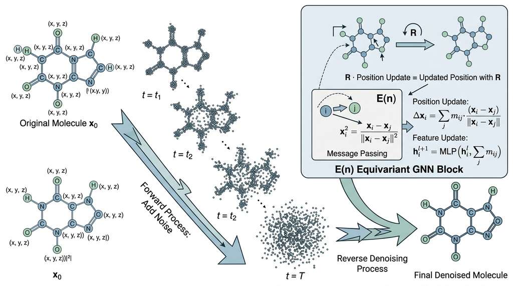
A molecule with \(n\) atoms is represented as a set of positions \(\mathbf{x} = [\mathbf{x}_1, \ldots, \mathbf{x}_n] \in \mathbb{R}^{n \times 3}\) and atomic features \(\mathbf{h} = [\mathbf{h}_1, \ldots, \mathbf{h}_n] \in \mathbb{R}^{n \times d}\) (one-hot atom types, charges, etc.). The forward diffusion process adds Gaussian noise to both positions and features:
$$q(\mathbf{x}_t, \mathbf{h}_t | \mathbf{x}_0, \mathbf{h}_0) = \mathcal{N}(\sqrt{\alpha_t}\, \mathbf{x}_0,\; (1-\alpha_t)\mathbf{I}) \cdot \mathcal{N}(\sqrt{\alpha_t}\, \mathbf{h}_0,\; (1-\alpha_t)\mathbf{I})$$The critical design choice is the denoising network \(\epsilon_\theta(\mathbf{x}_t, \mathbf{h}_t, t)\). Because molecular properties are invariant to rigid transformations (rotations, translations, reflections), the network must be equivariant: if we rotate the input positions by a rotation matrix \(\mathbf{R}\), the predicted position updates must rotate by the same \(\mathbf{R}\), while scalar predictions (atom types, charges) must remain unchanged:
$$\epsilon_\theta^{(\mathbf{x})}(\mathbf{R}\mathbf{x}_t, \mathbf{h}_t, t) = \mathbf{R}\, \epsilon_\theta^{(\mathbf{x})}(\mathbf{x}_t, \mathbf{h}_t, t)$$ $$\epsilon_\theta^{(\mathbf{h})}(\mathbf{R}\mathbf{x}_t, \mathbf{h}_t, t) = \epsilon_\theta^{(\mathbf{h})}(\mathbf{x}_t, \mathbf{h}_t, t)$$Checkpoint
So far: 3D molecular generation represents each molecule as a point cloud of atom positions and features, applies Gaussian noise via a forward diffusion process, and requires the denoising network to be equivariant so that rotated inputs produce correspondingly rotated outputs while scalar predictions stay unchanged.
EDM achieves this equivariance using an E(n) Equivariant Graph Neural Network (EGNN). Each layer updates node positions and features through equivariant message passing:
$$\mathbf{m}_{ij} = \phi_m(\mathbf{h}_i, \mathbf{h}_j, \|\mathbf{x}_i - \mathbf{x}_j\|^2, a_{ij})$$ $$\mathbf{x}_i' = \mathbf{x}_i + \sum_{j \neq i} (\mathbf{x}_i - \mathbf{x}_j) \cdot \phi_x(\mathbf{m}_{ij})$$ $$\mathbf{h}_i' = \phi_h\left(\mathbf{h}_i, \sum_{j \neq i} \mathbf{m}_{ij}\right)$$The position update is equivariant because it uses only relative displacements \((\mathbf{x}_i - \mathbf{x}_j)\) scaled by a learned scalar function \(\phi_x\). The feature update is invariant because it depends on positions only through the squared distance \(\|\mathbf{x}_i - \mathbf{x}_j\|^2\), which is rotation-invariant. Figure 49.1.1 illustrates Equivariant Diffusion Model (EDM) for 3D molecular generation.
Step-Through: One EGNN Message-Passing Update
Trace through a single EGNN layer on a toy two-atom molecule (atom A at position \(\mathbf{x}_A = (1, 0, 0)\) with feature \(\mathbf{h}_A = [1, 0]\) (carbon), atom B at \(\mathbf{x}_B = (0, 2, 0)\) with \(\mathbf{h}_B = [0, 1]\) (nitrogen)).
Step 1: Compute squared distance. \(\|\mathbf{x}_A - \mathbf{x}_B\|^2 = (1-0)^2 + (0-2)^2 + (0-0)^2 = 5\). This scalar is rotation-invariant: rotating both atoms by any angle preserves the value 5.
Step 2: Compute message. \(\mathbf{m}_{AB} = \phi_m([1,0],\; [0,1],\; 5)\). Suppose the MLP \(\phi_m\) outputs \(\mathbf{m}_{AB} = [0.3, -0.1]\).
Step 3: Update position of A. The displacement is \(\mathbf{x}_A - \mathbf{x}_B = (1, -2, 0)\). Suppose \(\phi_x(\mathbf{m}_{AB}) = 0.05\) (a learned scalar). New position: \(\mathbf{x}_A' = (1, 0, 0) + (1, -2, 0) \cdot 0.05 = (1.05, -0.10, 0)\). Atom A shifts slightly away from B along their connecting axis.
Step 4: Update feature of A. \(\mathbf{h}_A' = \phi_h([1, 0],\; [0.3, -0.1])\). Suppose the MLP outputs \(\mathbf{h}_A' = [0.9, 0.15]\). This depends only on the invariant message, not on absolute coordinates.
Equivariance check: rotate both atoms 90 degrees around the z-axis, so \(\mathbf{x}_A = (0, 1, 0)\), \(\mathbf{x}_B = (-2, 0, 0)\). The squared distance is still 5, messages are identical, and \(\phi_x\) produces the same 0.05. The displacement becomes \((2, 1, 0)\), so \(\mathbf{x}_A' = (0.10, 1.05, 0)\), which is exactly the 90-degree rotation of \((1.05, -0.10, 0)\). The geometry tracks correctly without retraining.
Mental Model
Think of equivariance like giving someone verbal directions to arrange furniture in a room. If you say "place the couch three feet from the wall, facing the fireplace," those instructions work regardless of whether the room faces north or south, because they describe relationships (distances and orientations between objects), not absolute GPS coordinates. An equivariant network works the same way: it learns to predict atomic positions using only the relative distances and directions between atoms, never their absolute coordinates in space. Rotating the entire molecule is like rotating the room; the relationships stay the same, so the network's predictions rotate along with the input automatically. A non-equivariant network, by contrast, would be like memorizing "the couch goes at coordinates (3, 7)" for every possible room orientation separately.
Equivariance is not just an aesthetic choice; it is a correctness requirement. A non-equivariant 3D generator would assign different likelihoods to rotated copies of the same molecule. In practice, this means the model would need to learn every possible orientation of every molecular motif separately, requiring vastly more training data. Equivariance builds physical symmetry into the architecture, allowing the model to generalize from a single orientation to all orientations automatically. This is the molecular analog of the translation equivariance that convolutions provide for images.
The following code demonstrates how to set up and sample from a pre-trained EDM model.
We use the e3_diffusion_for_molecules reference implementation.
import torch
from edm.models import EGNN_dynamics_QM9
from edm.sampling import sample_chain
from edm.utils import assert_mean_zero_with_mask


def sample_molecules_edm(
    model_path: str,
    n_samples: int = 10,
    n_atoms: int = 19,  # Max atoms for QM9-sized molecules
    device: str = "cuda",
) -> list[dict]:
    """Sample 3D molecules from a pre-trained EDM model.

    Returns list of dicts with 'positions' (n_atoms x 3),
    'atom_types' (n_atoms,), and 'charges' (n_atoms,).
    """
    # Load pre-trained model
    model = EGNN_dynamics_QM9.load_from_checkpoint(model_path)
    model = model.to(device).eval()

    # Sample atom counts from the training distribution
    # (QM9: molecules with up to 9 heavy atoms, ~29 atoms total including hydrogen)
    atom_counts = torch.full((n_samples,), n_atoms, device=device)

    # Create mask for variable-size molecules
    mask = torch.zeros(n_samples, n_atoms, device=device)
    for i, count in enumerate(atom_counts):
        mask[i, :count] = 1.0

    # Sample: reverse diffusion from noise to molecules
    with torch.no_grad():
        chain = sample_chain(
            model=model,
            n_samples=n_samples,
            n_nodes=n_atoms,
            node_mask=mask,
            n_steps=1000,       # Diffusion timesteps
            device=device,
        )

    # Extract final samples (t=0)
    positions = chain[-1]["positions"]   # (n_samples, n_atoms, 3)
    atom_types = chain[-1]["one_hot"]    # (n_samples, n_atoms, n_types)

    molecules = []
    for i in range(n_samples):
        n = int(atom_counts[i].item())
        molecules.append({
            "positions": positions[i, :n].cpu().numpy(),
            "atom_types": atom_types[i, :n].argmax(-1).cpu().numpy(),
            "n_atoms": n,
        })

    return molecules


# Post-process: convert to RDKit molecules for validation
from rdkit import Chem
from rdkit.Geometry import Point3D

ATOM_MAP = {0: 6, 1: 7, 2: 8, 3: 9}  # C, N, O, F for QM9

def edm_to_rdkit(mol_dict: dict) -> Chem.Mol:
    """Convert EDM output to an RDKit molecule with 3D coordinates."""
    rw_mol = Chem.RWMol()
    conf = Chem.Conformer(mol_dict["n_atoms"])

    for i in range(mol_dict["n_atoms"]):
        atomic_num = ATOM_MAP.get(mol_dict["atom_types"][i], 6)
        idx = rw_mol.AddAtom(Chem.Atom(atomic_num))
        pos = mol_dict["positions"][i]
        conf.SetAtomPosition(idx, Point3D(*pos.tolist()))

    rw_mol.AddConformer(conf, assignId=True)

    # Infer bonds from 3D distances using heuristic covalent radii
    Chem.rdDetermineBonds.DetermineBonds(rw_mol)

    return rw_mol.GetMol()
4. Structure-Based Generation with DiffSBDD
EDM generates molecules in a vacuum, with no awareness of the biological target. For drug design, we want to generate molecules that fit a specific protein binding pocket. DiffSBDD (Schneuing et al., 2023) extends equivariant diffusion to this setting by conditioning the generation process on the 3D structure of the protein pocket.
The pocket is represented as a point cloud of protein atom positions and features (atom type, residue type, backbone/sidechain flag). During denoising, the EGNN processes both ligand atoms (being denoised) and pocket atoms (fixed context) in the same graph. Cross-attention between ligand and pocket nodes allows the model to learn which molecular fragments complement which parts of the binding site:
$$\mathbf{m}_{ij}^{\text{cross}} = \phi_m^{\text{cross}}(\mathbf{h}_i^{\text{lig}}, \mathbf{h}_j^{\text{prot}}, \|\mathbf{x}_i^{\text{lig}} - \mathbf{x}_j^{\text{prot}}\|^2)$$The practical workflow involves three stages: (1) extract the binding pocket from a protein structure (typically residues within 10 Angstroms of a reference ligand), (2) run reverse diffusion conditioned on the pocket to generate candidate ligands, and (3) post-process generated molecules with bond inference, sanitization, and scoring.
from pathlib import Path
from Bio.PDB import PDBParser
import numpy as np


def extract_binding_pocket(
    pdb_path: str,
    ref_ligand_coords: np.ndarray,
    cutoff: float = 10.0,
) -> dict:
    """Extract protein pocket atoms within cutoff of reference ligand.

    Args:
        pdb_path: Path to protein PDB file.
        ref_ligand_coords: (n_lig_atoms, 3) coordinates of reference ligand.
        cutoff: Distance cutoff in Angstroms.

    Returns:
        Dict with 'positions', 'atom_types', 'residue_names'.
    """
    parser = PDBParser(QUIET=True)
    structure = parser.get_structure("protein", pdb_path)

    pocket_atoms = []
    for atom in structure.get_atoms():
        if atom.element in ("H", ""):
            continue
        coord = atom.get_vector().get_array()
        # Check if any ligand atom is within cutoff
        distances = np.linalg.norm(ref_ligand_coords - coord, axis=1)
        if distances.min() < cutoff:
            pocket_atoms.append({
                "position": coord,
                "element": atom.element,
                "residue": atom.get_parent().get_resname(),
            })

    return {
        "positions": np.array([a["position"] for a in pocket_atoms]),
        "elements": [a["element"] for a in pocket_atoms],
        "residues": [a["residue"] for a in pocket_atoms],
        "n_atoms": len(pocket_atoms),
    }


# Example: extract pocket from a kinase structure
pocket = extract_binding_pocket(
    pdb_path="data/4zau_protein.pdb",
    ref_ligand_coords=np.load("data/4zau_ligand_coords.npy"),
    cutoff=10.0,
)
print(f"Pocket: {pocket['n_atoms']} atoms from "
      f"{len(set(pocket['residues']))} unique residues")
A structural biology lab has solved the crystal structure of a previously undrugged enzyme implicated in neurodegeneration. No known inhibitors exist, so virtual screening against existing compound libraries yields no hits. They turn to DiffSBDD to generate molecules de novo for the newly resolved binding pocket.
They extract the pocket (238 protein atoms, 31 residues), run DiffSBDD to generate 1,000 candidate ligands, then filter: 847 pass valence checks, 612 have acceptable drug-likeness (Quantitative Estimate of Drug-likeness (QED) > 0.3), and 189 score below 4.0 on the synthetic accessibility scale. The top 50 are docked back into the pocket using conventional docking (AutoDock Vina) to verify binding pose consistency. Twelve molecules showing both high DiffSBDD confidence and favorable docking scores are advanced to synthesis planning with AiZynthFinder (Section 49.1.5).
5. Synthesizability and Retrosynthesis
A generated molecule is worthless if it cannot be synthesized. Two complementary approaches address this problem. Synthesizability scoring provides a fast, continuous estimate of how difficult a molecule is to make. The Synthetic Accessibility Score (SA Score) by Ertl and Schuffenhauer (2009) combines fragment contributions (frequent fragments are easy, rare fragments are hard) with a complexity penalty based on ring systems, stereocenters, and molecular size. SA scores range from 1 (trivially synthesizable) to 10 (essentially impossible), with most drug-like molecules falling between 2 and 5.
A low SA score tells you a molecule is plausible to make, but it does not tell you how; for that, you need a complete reaction plan working backward from the target to purchasable reagents.
Retrosynthetic analysis goes further, producing a complete synthetic route: a tree of reactions that transforms commercially available starting materials into the target molecule. AiZynthFinder (Genheden et al., 2020) uses Monte Carlo tree search (MCTS), a planning algorithm that balances exploration of untried reaction steps with exploitation of promising partial routes (see Section 45.2), to explore the space of possible disconnections, guided by a neural network that predicts which retrosynthetic templates apply to a given molecule. Each leaf of the search tree is a commercially available building block; a complete path from leaves to root is a viable synthetic route.
from aizynthfinder.aizynthfinder import AiZynthFinder


def plan_synthesis(smiles: str,
                   config_path: str = "aizynthfinder_config.yml",
                   time_limit: int = 120) -> dict:
    """Plan a retrosynthetic route for a target molecule.

    Args:
        smiles: Target molecule SMILES.
        config_path: Path to AiZynthFinder configuration.
        time_limit: Search time limit in seconds.

    Returns:
        Dict with route trees, scores, and building blocks.
    """
    finder = AiZynthFinder(configfile=config_path)
    finder.target_smiles = smiles
    finder.config.search.time_limit = time_limit

    # Run retrosynthetic search
    finder.tree_search()
    finder.build_routes()

    # Collect results
    routes = []
    for score, route in zip(finder.routes.scores, finder.routes):
        trees = route["trees"]
        building_blocks = set()
        for tree in trees:
            _collect_leaves(tree, building_blocks)

        routes.append({
            "score": round(score, 3),
            "n_steps": _count_steps(trees[0]),
            "building_blocks": list(building_blocks),
            "is_solved": all(
                _is_buyable(bb) for bb in building_blocks
            ),
        })

    return {
        "target": smiles,
        "n_routes": len(routes),
        "best_score": routes[0]["score"] if routes else None,
        "routes": routes[:5],  # Top 5 routes
    }


def _collect_leaves(tree: dict, leaves: set):
    """Recursively collect leaf SMILES from a route tree."""
    if "children" not in tree or not tree["children"]:
        leaves.add(tree["smiles"])
    else:
        for child in tree["children"]:
            _collect_leaves(child, leaves)


def _count_steps(tree: dict) -> int:
    """Count reaction steps in a route tree."""
    if "children" not in tree or not tree["children"]:
        return 0
    return 1 + max(_count_steps(c) for c in tree["children"])


def _is_buyable(smiles: str) -> bool:
    """Check if a building block is commercially available."""
    # In production, query a vendor database (Enamine, Sigma-Aldrich)
    # Here we use a simple molecular weight heuristic
    from rdkit import Chem
    from rdkit.Chem import Descriptors
    mol = Chem.MolFromSmiles(smiles)
    if mol is None:
        return False
    return Descriptors.MolWt(mol) < 300  # Simple heuristic
Real-World Application: Insilico Medicine's Drug Discovery Pipeline
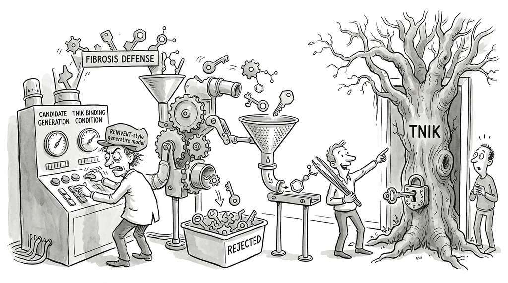
Insilico Medicine used a REINVENT-style generative model combined with structure-based filtering to design a novel inhibitor of the fibrosis target TNIK (TRAF2 and NCK interacting kinase). The system generated candidates conditioned on the TNIK binding pocket, scored them with an ensemble of QSAR models, and filtered for synthetic accessibility. The resulting molecule, INS018_055, advanced from AI-generated hit to Phase II clinical trials in under 30 months, roughly a third of what industry benchmarks typically report for early-stage drug discovery, making it one of the first publicly disclosed AI-designed drugs to reach Phase II in humans.
The molecular operations scattered throughout this section (SMILES parsing, fingerprint computation, substructure matching, property calculation) are all handled by RDKit in one to three lines each. Without RDKit, implementing SMILES parsing alone would require thousands of lines of grammar code. RDKit provides over 200 molecular descriptors, substructure search via SMARTS patterns, 2D/3D coordinate generation, conformer sampling, and reaction handling. It is to cheminformatics what NumPy is to numerical computing: the foundation everything else builds on.
from rdkit import Chem
from rdkit.Chem import AllChem, Descriptors, QED

mol = Chem.MolFromSmiles("CC(=O)Oc1ccccc1C(=O)O")  # Aspirin
print(f"MW: {Descriptors.MolWt(mol):.1f}")          # 180.2
print(f"LogP: {Descriptors.MolLogP(mol):.2f}")       # 1.31
print(f"QED: {QED.qed(mol):.3f}")                    # 0.550
print(f"TPSA: {Descriptors.TPSA(mol):.1f}")          # 63.6
fp = AllChem.GetMorganFingerprintAsBitVect(mol, 2, nBits=2048)
6. ChemCrow: LLM-Augmented Chemistry
ChemCrow (Bran et al., 2023) takes a different approach to molecular generation: instead of training a specialized generative model, it augments a large language model with chemistry-specific tools. ChemCrow wraps GPT-4 with a toolkit of 18 chemistry tools (as of 2025, successors such as ChemAgent and Coscientist have adopted newer LLM backends including GPT-4o and Claude, with expanded tool sets; the architectural pattern, however, remains the same) including RDKit operations, web searches for safety data, reaction prediction APIs, and molecular property calculators. The LLM acts as a reasoning engine that plans multi-step chemical tasks by composing tool calls.
ChemCrow instantiates the research agent paradigm from Chapter 40, with a chemistry-specific MCP server (Chapter 12). Its advantage over pure generative models is interpretability: ChemCrow explains its reasoning, cites sources, and decomposes complex tasks into verifiable steps. The trade-off is throughput, since an LLM tool-use loop produces one molecule in seconds while a SMILES generator produces thousands per second.
from langchain.agents import AgentExecutor, create_react_agent
from langchain_openai import ChatOpenAI
from langchain.tools import Tool
from rdkit import Chem
from rdkit.Chem import Descriptors, QED


# Define chemistry tools for the LLM agent
def smiles_validity_tool(smiles: str) -> str:
    """Check if a SMILES string represents a valid molecule."""
    mol = Chem.MolFromSmiles(smiles)
    if mol is None:
        return f"Invalid SMILES: {smiles}"
    canonical = Chem.MolToSmiles(mol)
    return f"Valid. Canonical SMILES: {canonical}, Formula: {Chem.rdMolDescriptors.CalcMolFormula(mol)}"


def property_calculator_tool(smiles: str) -> str:
    """Calculate drug-relevant properties for a molecule."""
    mol = Chem.MolFromSmiles(smiles)
    if mol is None:
        return "Invalid SMILES"
    props = {
        "MW": f"{Descriptors.MolWt(mol):.1f}",
        "LogP": f"{Descriptors.MolLogP(mol):.2f}",
        "HBD": Descriptors.NumHDonors(mol),
        "HBA": Descriptors.NumHAcceptors(mol),
        "TPSA": f"{Descriptors.TPSA(mol):.1f}",
        "QED": f"{QED.qed(mol):.3f}",
        "RotBonds": Descriptors.NumRotatableBonds(mol),
        "Rings": Chem.rdMolDescriptors.CalcNumRings(mol),
    }
    return "\n".join(f"  {k}: {v}" for k, v in props.items())


def similarity_search_tool(query: str) -> str:
    """Find similar molecules (placeholder for database search)."""
    # In production: query ChEMBL, PubChem, or internal databases
    return f"Similarity search for '{query}': [placeholder for DB results]"


tools = [
    Tool(name="CheckSMILES", func=smiles_validity_tool,
         description="Validate a SMILES string and get canonical form"),
    Tool(name="CalcProperties", func=property_calculator_tool,
         description="Calculate molecular properties from SMILES"),
    Tool(name="SimilaritySearch", func=similarity_search_tool,
         description="Find structurally similar known molecules"),
]

# Create a ReAct agent with chemistry tools
llm = ChatOpenAI(model="gpt-4", temperature=0)
# agent = create_react_agent(llm, tools, prompt=chemistry_prompt)
# executor = AgentExecutor(agent=agent, tools=tools, verbose=True)
# result = executor.invoke({"input": "Suggest modifications to aspirin ..."})
Research Frontier
In 2024, Abramson et al. introduced AlphaFold 3 (Nature, 2024), which extends structure prediction beyond proteins to jointly model protein, nucleic acid, small molecule, ion, and post-translational modification complexes using a unified diffusion architecture. Unlike earlier docking or cofolding tools that treat ligand and protein separately, AlphaFold 3 predicts the full biomolecular assembly in a single forward pass, achieving state-of-the-art accuracy on protein-ligand binding pose prediction (surpassing traditional docking methods on the PoseBusters benchmark). For molecular generation, this is transformative: structure-based generators like DiffSBDD can now condition on AlphaFold 3-predicted pocket geometries even when no experimental crystal structure exists, dramatically expanding the space of druggable targets. The system also highlights a remaining gap: while pose prediction has improved substantially, binding affinity ranking remains unreliable, and generated molecules still require experimental validation.
Try It: Score and Rank a Molecular Library
Build a mini drug-likeness scoring pipeline from scratch using only RDKit and standard
Python libraries. (1) Install RDKit: pip install rdkit (or
conda install -c conda-forge rdkit). (2) Download a small set of bioactive
molecules from ChEMBL: visit https://www.ebi.ac.uk/chembl/, search for a
target of interest (e.g., "EGFR"), and export 50-100 compound SMILES as a CSV file.
(3) Write a Python script that reads the CSV, parses each SMILES with
Chem.MolFromSmiles(), and computes QED, SA Score, LogP, molecular weight,
and number of hydrogen bond donors/acceptors for every valid molecule. (4) Rank the
molecules by the composite MPO score (geometric mean of normalized component scores,
as shown in the compute_mpo_score function in this section) and print the
top 10 candidates. (5) For each top candidate, check Lipinski's Rule of Five violations
(MW < 500, LogP < 5, HBD <= 5, HBA <= 10) and flag any that fail two or
more rules. Compare your top-ranked molecules against the original ChEMBL activity data
to see whether high MPO scores correlate with reported potency.
The Billion-Dollar Typo
SMILES notation is so syntactically fragile that changing a single character can turn a harmless molecule into a potent toxin, or vice versa. In 2020, a team at MIT trained a SMILES-based generator to optimize for predicted antimicrobial activity and discovered halicin, a molecule structurally unlike any existing antibiotic, which proved effective against drug-resistant bacteria in mice. The catch: halicin sits only a few SMILES characters away from molecules flagged as potential chemical weapons by the same model. When the researchers later reversed their objective function (maximizing predicted toxicity instead of minimizing it), the generator produced 40,000 plausible toxic molecules in under six hours, many resembling known nerve agents. The episode prompted a community-wide debate about dual-use risks in molecular generation, and the paper describing the toxicity experiment (Urbina et al., Nature Machine Intelligence, 2022) was published specifically as a warning.
Lab: Build a SMILES Diversity Explorer
Goal: Understand how Morgan fingerprints (circular substructure fingerprints that encode each atom's neighborhood up to a given bond radius as a fixed-length bit vector) and Tanimoto similarity define "diversity" in a chemical library, the same metric used to prevent mode collapse in REINVENT.
Tools needed: Python 3.8+, rdkit (pip install rdkit),
matplotlib, scikit-learn. About 20 minutes.
Procedure: (1) Collect 100 drug SMILES from the freely downloadable
DrugBank "approved drugs" list or from ChEMBL. (2) For each molecule, compute a Morgan
fingerprint (radius 2, 2048 bits) using
AllChem.GetMorganFingerprintAsBitVect(mol, 2, nBits=2048).
(3) Build a 100x100 pairwise Tanimoto similarity matrix. (4) Apply t-SNE
(sklearn.manifold.TSNE) to the fingerprint bit vectors and plot the 2D
embedding, coloring points by a molecular property of your choice (e.g., QED or LogP).
(5) Identify the two most similar and two most dissimilar pairs. Visualize them with
Draw.MolsToGridImage() and inspect whether fingerprint similarity matches
your chemical intuition.
What to vary: Change the fingerprint radius (1, 2, 3) and bit length
(512, 1024, 2048, 4096). Observe how the similarity distribution shifts: larger radii
capture more context and push similarities lower.
What to observe: At radius 1 many structurally different drugs appear
"similar" (Tanimoto > 0.5); at radius 3 almost everything drops below 0.3. This
calibration is essential when setting the max_similarity threshold in
scaffold-hopping reward functions.
What's Next
Generating candidate molecules is only half the battle. The next section, Section 49.2: Protein-Ligand Cofolding, addresses the complementary question: once we have a candidate ligand, how do we predict whether it will actually bind the target protein, in what pose, and with what affinity? We will see how Boltz-1 and Chai-1 replace the traditional docking-then-scoring pipeline with end-to-end learned structure prediction, and how DiffDock-L frames pose prediction as a generative process.