39.2 AI-Generated Hypotheses

The Big Picture

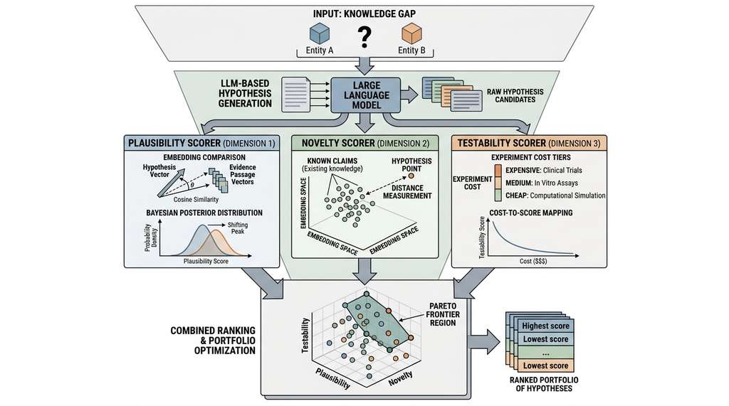
Gap analysis tells us where hypotheses might live. This section addresses how to generate them and how to evaluate them. We use large language models (LLMs) as hypothesis generators, grounding their output in retrieved scientific context to prevent hallucination. We then develop three orthogonal scoring dimensions: plausibility (consistency with existing evidence), novelty (distance from known claims in embedding space), and testability (estimated cost and feasibility of experimental verification). These scores transform a raw list of LLM-generated statements into a ranked portfolio of research directions, ready for human review or autonomous pursuit by the research agents of Chapter 40. Figure 39.2.1 illustrates hypothesis scoring pipeline with three orthogonal dimensions.

1. From Gaps to Hypotheses: LLM-Based Generation

In 2003, two proteins sat three hops apart in a yeast interaction network. No published paper linked them; no shared pathway annotation connected them. A decade later, researchers confirmed they co-regulate the same stress-response cascade. Today, an LLM can ingest the same literature, flag that structural gap, and propose a candidate mechanistic link in seconds, compressing a decade of literature synthesis into a single API call. The question is no longer whether machines can generate scientific hypotheses. It is how to ensure those hypotheses are specific enough to test, grounded enough to trust, and novel enough to matter.

A structured prompting pipeline sequences LLM interactions so that each stage has a distinct role and a constrained output format, unlike a single open-ended prompt. It matters because unconstrained generation produces text that reads well but lacks the internal structure (explicit mechanisms, falsifiable predictions, stated assumptions) needed for scientific evaluation. The pipeline first retrieves relevant literature passages. It then prompts the LLM to generate hypotheses that conform to a rigid JSON schema enforcing each required field. Finally, a self-critique stage flags weaknesses in each candidate. Use a structured pipeline rather than free-form generation whenever hypotheses must be machine-scored or fed into downstream automation; use free-form generation only for early brainstorming where volume matters more than rigor.

Without structure, LLM-generated hypotheses fail silently: they read like real science but lack falsifiable predictions, so labs waste months designing experiments around claims that were never precise enough to test. That failure mode makes the next mechanism essential.

The challenge is to channel LLM generation toward hypotheses that are genuinely useful, not just plausible-sounding text. We achieve this through a structured prompting pipeline with three stages: context retrieval, constrained generation, and self-critique. Figure 39.5 illustrates the complete flow from retrieved literature through scored hypotheses. In short: structure turns fluent text into something a scientist can actually bring to the bench.

import anthropic
import json
from dataclasses import dataclass, field


@dataclass
class Hypothesis:
    """A generated scientific hypothesis with metadata."""
    statement: str
    domain: str
    mechanism: str
    supporting_evidence: list[str]
    predictions: list[str]
    assumptions: list[str]
    plausibility_score: float = 0.0
    novelty_score: float = 0.0
    testability_score: float = 0.0


HYPOTHESIS_SYSTEM_PROMPT = """You are a scientific hypothesis generator.
Given a knowledge gap (two entities that may be related but have no
documented connection) and supporting context from the scientific
literature, generate a concrete, testable hypothesis.

Your hypothesis must include:
1. A clear statement of the proposed relationship
2. A plausible mechanism connecting the entities
3. Specific, falsifiable predictions
4. Explicit assumptions that must hold

Respond in JSON with this schema:
{
  "statement": "The hypothesis in one sentence",
  "domain": "Scientific domain (e.g., molecular biology, materials science)",
  "mechanism": "Proposed causal mechanism in 2-3 sentences",
  "supporting_evidence": ["Evidence point 1", "Evidence point 2", ...],
  "predictions": ["Testable prediction 1", "Testable prediction 2", ...],
  "assumptions": ["Assumption 1", "Assumption 2", ...]
}

Rules:
- Be specific: name concrete entities, pathways, and measurable outcomes.
- Be honest about uncertainty: flag speculative steps in the mechanism.
- Generate predictions that could FAIL: a hypothesis that cannot be
  falsified is not a scientific hypothesis.
- Do not generate hypotheses that are already established knowledge."""


def generate_hypotheses(
    entity_a: str,
    entity_b: str,
    context_passages: list[str],
    n_hypotheses: int = 5,
    model: str = "claude-sonnet-4-20250514",
) -> list[Hypothesis]:
    """Generate hypotheses for a knowledge gap using Claude.

    Args:
        entity_a: First entity in the gap.
        entity_b: Second entity in the gap.
        context_passages: Retrieved passages about both entities.
        n_hypotheses: Number of hypotheses to generate.
        model: Anthropic model to use.

    Returns:
        List of generated Hypothesis objects.
    """
    client = anthropic.Anthropic()

    context_block = "\n\n".join(
        f"[Passage {i+1}]: {p}" for i, p in enumerate(context_passages)
    )

    user_prompt = f"""Knowledge gap detected between:
- Entity A: {entity_a}
- Entity B: {entity_b}

Supporting context from the literature:
{context_block}

Generate {n_hypotheses} distinct hypotheses about the potential
relationship between {entity_a} and {entity_b}. Each hypothesis
should propose a DIFFERENT mechanism or relationship type.
Return a JSON array of hypothesis objects."""

    response = client.messages.create(
        model=model,
        max_tokens=4096,
        system=HYPOTHESIS_SYSTEM_PROMPT,
        messages=[{"role": "user", "content": user_prompt}],
    )

    # Parse the structured output
    text = response.content[0].text
    # Extract JSON from potential markdown code fences
    if "```json" in text:
        text = text.split("```json")[1].split("```")[0]
    elif "```" in text:
        text = text.split("```")[1].split("```")[0]

    raw_hypotheses = json.loads(text)
    if isinstance(raw_hypotheses, dict):
        raw_hypotheses = [raw_hypotheses]

    return [
        Hypothesis(
            statement=h["statement"],
            domain=h.get("domain", "unknown"),
            mechanism=h.get("mechanism", ""),
            supporting_evidence=h.get("supporting_evidence", []),
            predictions=h.get("predictions", []),
            assumptions=h.get("assumptions", []),
        )
        for h in raw_hypotheses
    ]

2. Self-Critique and Refinement

Raw LLM-generated hypotheses often have weaknesses: vague mechanisms, predictions that are too easy to confirm, or implicit assumptions that are actually false. A self-critique step uses the same LLM (or a more capable model) to identify and address these weaknesses before scoring:

CRITIQUE_PROMPT = """You are a scientific reviewer evaluating a hypothesis.

Hypothesis: {statement}
Mechanism: {mechanism}
Predictions: {predictions}

Critique this hypothesis on four dimensions:
1. SPECIFICITY: Are the entities and mechanisms named concretely enough
   to design an experiment?
2. FALSIFIABILITY: Could the predictions actually fail? A prediction
   like "gene expression may change" is not falsifiable.
3. MECHANISM: Is the proposed causal chain plausible given known
   biology/chemistry/physics? Identify any steps that require
   unknown or speculative interactions.
4. NOVELTY: Is this genuinely new, or is it a restatement of
   known results?

Return JSON:
{{
  "critique": "2-3 sentence summary of weaknesses",
  "specificity_ok": true/false,
  "falsifiable": true/false,
  "mechanism_gaps": ["gap 1", ...],
  "is_novel": true/false,
  "refined_statement": "Improved version of the hypothesis",
  "refined_predictions": ["More specific prediction 1", ...]
}}"""


def critique_and_refine(
    hypothesis: Hypothesis,
    model: str = "claude-sonnet-4-20250514",
) -> Hypothesis:
    """Apply self-critique to improve a hypothesis.

    Returns a refined version with more specific predictions
    and explicit mechanism gaps.
    """
    client = anthropic.Anthropic()

    response = client.messages.create(
        model=model,
        max_tokens=2048,
        messages=[{
            "role": "user",
            "content": CRITIQUE_PROMPT.format(
                statement=hypothesis.statement,
                mechanism=hypothesis.mechanism,
                predictions=json.dumps(hypothesis.predictions),
            ),
        }],
    )

    text = response.content[0].text
    if "```json" in text:
        text = text.split("```json")[1].split("```")[0]
    elif "```" in text:
        text = text.split("```")[1].split("```")[0]

    critique = json.loads(text)

    # Update hypothesis with refined versions
    refined = Hypothesis(
        statement=critique.get("refined_statement", hypothesis.statement),
        domain=hypothesis.domain,
        mechanism=hypothesis.mechanism,
        supporting_evidence=hypothesis.supporting_evidence,
        predictions=critique.get(
            "refined_predictions", hypothesis.predictions
        ),
        assumptions=hypothesis.assumptions + critique.get(
            "mechanism_gaps", []
        ),
    )
    return refined

Once each hypothesis has been sharpened through self-critique, the next step is to quantify how well it holds up against what science already knows, starting with plausibility.

3. Scoring Dimension 1: Plausibility

A plausible hypothesis is one that is consistent with existing evidence. We quantify plausibility using two complementary signals: the semantic consistency of the hypothesis with retrieved literature, and a Bayesian estimate of the hypothesis's prior probability given the evidence.

For semantic consistency, we compute the average cosine similarity (where cosine similarity is the dot product of two unit-length vectors, ranging from −1 for opposite meanings to +1 for identical meanings) between the hypothesis embedding (a fixed-length numeric vector that captures the semantic meaning of a text passage) and the embeddings of the supporting context passages. A hypothesis that aligns well with the literature (high similarity) is more plausible than one that contradicts it (low similarity), though extremely high similarity may indicate redundancy rather than novelty (a tension we resolve in the combined scoring of Section 39.3).

Bayesian Evidence Accumulation

For Bayesian plausibility, we use PyMC to estimate the posterior probability of the hypothesis given the evidence. The model treats each piece of evidence as a noisy observation of the hypothesis's truth:

where \(P(H)\) is the prior probability (set by the structural gap score from Section 39.1), and \(P(E_i \mid H)\) is the likelihood of observing evidence \(E_i\) if hypothesis \(H\) is true. We model each evidence term as a Bernoulli trial with a relevance-weighted probability:

where \(\text{sim}\) is cosine similarity, \(\mathbf{e}_{E_i}\) and \(\mathbf{e}_H\) are the embedding vectors of evidence passage \(E_i\) and hypothesis \(H\) respectively, and \(\beta\) controls how sharply similarity translates into evidential support. Higher \(\beta\) makes the scoring more selective; lower \(\beta\) treats all moderately relevant evidence as equally supportive.

import pymc as pm
import numpy as np
from sentence_transformers import SentenceTransformer


class PlausibilityScorer:
    """Score hypothesis plausibility using embedding similarity
    and Bayesian evidence accumulation."""

    def __init__(self, model_name: str = "all-MiniLM-L6-v2"):
        self.embedder = SentenceTransformer(model_name)

    def semantic_consistency(
        self,
        hypothesis: str,
        evidence_passages: list[str],
    ) -> float:
        """Cosine similarity between hypothesis and evidence."""
        all_texts = [hypothesis] + evidence_passages
        embeddings = self.embedder.encode(all_texts, normalize_embeddings=True)

        h_emb = embeddings[0]
        e_embs = embeddings[1:]

        similarities = e_embs @ h_emb
        return float(np.mean(similarities))

    def bayesian_plausibility(
        self,
        hypothesis: str,
        evidence_passages: list[str],
        prior_gap_score: float = 0.5,
        beta: float = 2.0,
    ) -> float:
        """Bayesian posterior estimate of hypothesis plausibility.

        Args:
            hypothesis: The hypothesis statement.
            evidence_passages: Supporting evidence texts.
            prior_gap_score: Prior from structural gap analysis (0 to 1).
            beta: Sharpness of the similarity-to-likelihood mapping.

        Returns:
            Posterior plausibility score (0 to 1).
        """
        # Compute similarities as evidence strengths
        all_texts = [hypothesis] + evidence_passages
        embeddings = self.embedder.encode(all_texts, normalize_embeddings=True)
        h_emb = embeddings[0]
        e_embs = embeddings[1:]
        similarities = np.clip(e_embs @ h_emb, 0.0, 1.0)

        # Bayesian model: each evidence piece is a noisy indicator
        with pm.Model() as model:
            # Prior: informed by structural gap score
            h_true = pm.Beta("h_true", alpha=prior_gap_score * 10 + 1,
                             beta=(1 - prior_gap_score) * 10 + 1)

            # Likelihood: evidence relevance given hypothesis truth
            for i, sim in enumerate(similarities):
                # 0.1 baseline: even irrelevant evidence has a small
            # chance of appearing in the corpus by coincidence
            likelihood = h_true * sim**beta + (1 - h_true) * 0.1
                pm.Bernoulli(f"e_{i}", p=likelihood, observed=1)

            # Sample posterior
            trace = pm.sample(
                1000, tune=500, cores=1,
                return_inferencedata=False,
                progressbar=False,
            )

        posterior_mean = float(np.mean(trace["h_true"]))
        return posterior_mean

    def score(
        self,
        hypothesis: str,
        evidence_passages: list[str],
        prior_gap_score: float = 0.5,
    ) -> float:
        """Combined plausibility score (0 to 1)."""
        sem = self.semantic_consistency(hypothesis, evidence_passages)
        bay = self.bayesian_plausibility(
            hypothesis, evidence_passages, prior_gap_score
        )
        # Geometric mean: penalizes candidates that score
        # near zero on either signal, unlike an arithmetic
        # mean which lets a high score on one mask a low score
        # on the other
        return float(np.sqrt(sem * bay))

4. Scoring Dimension 2: Novelty as Embedding Distance

A novel hypothesis says something that existing knowledge does not. We operationalize novelty as the distance between the hypothesis embedding and the nearest existing claim in our knowledge base. If a hypothesis is very close to something already published, it is a restatement; if it is very far from everything known, it is either genuinely novel or nonsensical (a distinction resolved by the plausibility score).

Formally, given a hypothesis embedding \(\mathbf{h}\) and a database of known claim embeddings \(\{\mathbf{c}_1, \ldots, \mathbf{c}_m\}\), the novelty score is:

where \(\text{sim}\) is cosine similarity. A score near 0 means the hypothesis is a near-exact match to something known; a score near 1 means it is far from anything in the database. We compute this efficiently using Qdrant:

import numpy as np
from qdrant_client import QdrantClient
from qdrant_client.models import Distance, VectorParams, PointStruct
from sentence_transformers import SentenceTransformer


class NoveltyScorer:
    """Score hypothesis novelty as embedding distance from known claims."""

    def __init__(
        self,
        known_claims: list[str],
        model_name: str = "all-MiniLM-L6-v2",
        collection_name: str = "known_claims",
    ):
        self.embedder = SentenceTransformer(model_name)
        self.client = QdrantClient(":memory:")
        self.collection_name = collection_name

        # Embed and index all known claims
        embeddings = self.embedder.encode(
            known_claims, normalize_embeddings=True
        )
        dim = embeddings.shape[1]

        self.client.create_collection(
            collection_name=collection_name,
            vectors_config=VectorParams(
                size=dim, distance=Distance.COSINE
            ),
        )

        points = [
            PointStruct(
                id=i,
                vector=emb.tolist(),
                payload={"claim": claim},
            )
            for i, (claim, emb) in enumerate(zip(known_claims, embeddings))
        ]
        self.client.upsert(collection_name=collection_name, points=points)

    def score(self, hypothesis: str, k: int = 5) -> dict:
        """Compute novelty score for a hypothesis.

        Args:
            hypothesis: The hypothesis statement.
            k: Number of nearest claims to retrieve for context.

        Returns:
            Dict with novelty_score and nearest_claims.
        """
        h_emb = self.embedder.encode(
            [hypothesis], normalize_embeddings=True
        )[0]

        results = self.client.search(
            collection_name=self.collection_name,
            query_vector=h_emb.tolist(),
            limit=k,
        )

        if not results:
            return {"novelty_score": 1.0, "nearest_claims": []}

        max_similarity = results[0].score
        novelty = 1.0 - max_similarity

        nearest = [
            {
                "claim": r.payload["claim"],
                "similarity": r.score,
            }
            for r in results
        ]

        return {
            "novelty_score": float(novelty),
            "nearest_claims": nearest,
        }

5. Scoring Dimension 3: Testability as Experiment Cost

A testable hypothesis is one that can be confirmed or refuted through a feasible experiment. We decompose testability into three components: (1) whether the predictions are operationally measurable, (2) the estimated cost and time of the required experiment, and (3) the statistical power achievable with practical sample sizes.

The first component (measurability) we delegate to the LLM, which has domain knowledge about what can and cannot be measured with current technology. The second component (experiment cost) we estimate using a lookup table of typical experimental costs by assay type, augmented by LLM reasoning for novel assay designs. The third component (statistical power) we compute analytically for standard experimental designs:

where \(n\) is the required sample size per group, \(\delta\) is the minimum detectable effect size, \(\sigma\) is the expected standard deviation, and \(z_{\alpha/2}\), \(z_{\beta}\) are the critical values for significance level \(\alpha\) and power \(1-\beta\).

import anthropic
import json
import math
from dataclasses import dataclass


@dataclass
class TestabilityAssessment:
    """Assessment of how testable a hypothesis is."""
    measurable: bool
    experiment_type: str
    estimated_cost_usd: float
    estimated_duration_days: int
    required_sample_size: int
    statistical_power: float
    testability_score: float  # Combined score 0-1
    reasoning: str


# Typical costs by experiment type (order-of-magnitude estimates)
EXPERIMENT_COSTS = {
    "computational_simulation": {"cost_per_run": 10, "time_days": 1},
    "cell_culture_assay": {"cost_per_run": 500, "time_days": 14},
    "animal_model": {"cost_per_run": 5000, "time_days": 90},
    "clinical_trial_phase1": {"cost_per_run": 1_000_000, "time_days": 365},
    "survey_study": {"cost_per_run": 50, "time_days": 30},
    "materials_synthesis": {"cost_per_run": 1000, "time_days": 7},
    "spectroscopy_measurement": {"cost_per_run": 200, "time_days": 1},
    "genomics_sequencing": {"cost_per_run": 300, "time_days": 7},
    "proteomics_mass_spec": {"cost_per_run": 800, "time_days": 14},
    "behavioral_experiment": {"cost_per_run": 100, "time_days": 60},
}


def required_sample_size(
    effect_size: float,
    std_dev: float = 1.0,
    alpha: float = 0.05,
    power: float = 0.8,
) -> int:
    """Compute required sample size for a two-group comparison.

    Uses the standard formula for a two-sample t-test.
    """
    from scipy import stats
    z_alpha = stats.norm.ppf(1 - alpha / 2)
    z_beta = stats.norm.ppf(power)
    n = math.ceil((z_alpha + z_beta)**2 * 2 * std_dev**2 / effect_size**2)
    return max(n, 3)  # Minimum 3 per group


def assess_testability(
    hypothesis: str,
    predictions: list[str],
    model: str = "claude-sonnet-4-20250514",
) -> TestabilityAssessment:
    """Assess hypothesis testability using LLM reasoning
    and analytical cost estimation.

    Args:
        hypothesis: The hypothesis statement.
        predictions: Testable predictions from the hypothesis.
        model: Anthropic model for experiment design reasoning.

    Returns:
        TestabilityAssessment with cost, duration, and score.
    """
    client = anthropic.Anthropic()

    prompt = f"""Assess the testability of this scientific hypothesis.

Hypothesis: {hypothesis}
Predictions: {json.dumps(predictions)}

Determine:
1. Can the predictions be measured with current technology? (yes/no)
2. What type of experiment is needed? Choose from:
   {json.dumps(list(EXPERIMENT_COSTS.keys()))}
3. What is the expected effect size (Cohen's d)?
   Small = 0.2, Medium = 0.5, Large = 0.8
4. Brief reasoning (2-3 sentences).

Return JSON:
{{"measurable": true/false, "experiment_type": "...",
  "effect_size": 0.5, "reasoning": "..."}}"""

    response = client.messages.create(
        model=model,
        max_tokens=1024,
        messages=[{"role": "user", "content": prompt}],
    )

    text = response.content[0].text
    if "```json" in text:
        text = text.split("```json")[1].split("```")[0]
    elif "```" in text:
        text = text.split("```")[1].split("```")[0]

    assessment = json.loads(text)

    # Look up experiment costs
    exp_type = assessment.get("experiment_type", "computational_simulation")
    costs = EXPERIMENT_COSTS.get(exp_type, EXPERIMENT_COSTS["computational_simulation"])

    # Compute required sample size
    effect_size = assessment.get("effect_size", 0.5)
    n = required_sample_size(effect_size)

    total_cost = costs["cost_per_run"] * n
    duration = costs["time_days"]

    # Testability score: inverse log of cost, normalized
    # Cheaper and faster experiments are more testable
    max_cost = 10_000_000  # $10M as upper bound
    cost_score = 1.0 - math.log10(total_cost + 1) / math.log10(max_cost)
    cost_score = max(0.0, min(1.0, cost_score))

    measurable = assessment.get("measurable", False)
    testability = cost_score * (1.0 if measurable else 0.1)

    return TestabilityAssessment(
        measurable=measurable,
        experiment_type=exp_type,
        estimated_cost_usd=total_cost,
        estimated_duration_days=duration,
        required_sample_size=n,
        statistical_power=0.8,  # Fixed target
        testability_score=testability,
        reasoning=assessment.get("reasoning", ""),
    )

With all three automated scores in hand, the pipeline can rank hundreds of candidates in minutes; yet no scoring formula captures the practical constraints that only a domain expert knows, which is why the final stage puts the scientist back in control.

6. Human-AI Refinement Loops

Automated scoring provides a first-pass ranking, but the most productive hypothesis generation systems keep the human scientist in the loop. The AI generates and scores; the human provides domain expertise, experimental intuition, and strategic direction. The iterative refinement cycle below formalizes this collaboration:

from dataclasses import dataclass


@dataclass
class RefinementFeedback:
    """Human feedback on a generated hypothesis."""
    hypothesis_id: int
    action: str  # "accept", "reject", "refine"
    comment: str
    refined_statement: str | None = None
    priority: int = 0  # 1-5, scientist's subjective ranking


def apply_refinement(
    hypotheses: list[Hypothesis],
    feedback: list[RefinementFeedback],
    model: str = "claude-sonnet-4-20250514",
) -> list[Hypothesis]:
    """Apply human feedback to refine generated hypotheses.

    Processes scientist feedback through the LLM to produce
    improved hypothesis versions.
    """
    client = anthropic.Anthropic()
    refined = []

    for fb in feedback:
        if fb.action == "reject":
            continue  # Drop rejected hypotheses

        h = hypotheses[fb.hypothesis_id]

        if fb.action == "accept":
            h.plausibility_score += 0.1  # Human endorsement bonus
            refined.append(h)
            continue

        if fb.action == "refine":
            # Use the scientist's comment to guide LLM refinement
            prompt = f"""A scientist reviewed this hypothesis and
provided feedback. Refine the hypothesis accordingly.

Original: {h.statement}
Mechanism: {h.mechanism}
Feedback: {fb.comment}
{f"Scientist's revised statement: {fb.refined_statement}" if fb.refined_statement else ""}

Generate a refined hypothesis in JSON format with the same
schema as the original (statement, mechanism, predictions,
assumptions)."""

            response = client.messages.create(
                model=model,
                max_tokens=2048,
                messages=[{"role": "user", "content": prompt}],
            )

            text = response.content[0].text
            if "```json" in text:
                text = text.split("```json")[1].split("```")[0]
            elif "```" in text:
                text = text.split("```")[1].split("```")[0]

            data = json.loads(text)
            refined_h = Hypothesis(
                statement=data.get("statement", h.statement),
                domain=h.domain,
                mechanism=data.get("mechanism", h.mechanism),
                supporting_evidence=h.supporting_evidence,
                predictions=data.get("predictions", h.predictions),
                assumptions=data.get("assumptions", h.assumptions),
            )
            refined.append(refined_h)

    return refined

The refinement loop addresses a fundamental limitation of automated generation: LLMs lack the scientist's tacit knowledge of lab capabilities, available collaborators, and aligned funding calls. By injecting this context, the scientist transforms a generic hypothesis list into a personalized research strategy.

Exercises

1. (Conceptual) The novelty score measures distance from known claims in embedding space. But embedding models have finite resolution: two genuinely different hypotheses might have similar embeddings if their surface wording is similar. Design a novelty scoring method that is more sensitive to semantic differences. Consider using the predictions rather than the statement as the basis for novelty comparison, and explain why this might better capture scientific novelty.
2. (Coding) Implement an A/B test of two hypothesis generation prompts: one that asks the LLM to "be creative and generate surprising hypotheses" versus one that asks it to "identify the most likely missing connections based on the evidence." Generate 20 hypotheses with each prompt for the same set of knowledge gaps, score them on all three dimensions, and compare the distributions. Which prompt strategy produces better hypotheses, and by which metric?
3. (Analysis) The Bayesian plausibility model treats each evidence passage as an independent observation. In reality, evidence passages from the same paper or research group are correlated. Extend the PyMC model to include a hierarchical structure where evidence passages are grouped by source, with a shared noise parameter per source. How does this change the posterior plausibility estimates compared to the independence assumption?