39.3 Building a Hypothesis Generator

1. Pipeline Architecture

What if you could hand a computer a graph of everything science knows about neurodegeneration, walk away for ten minutes, and come back to a ranked shortlist of testable hypotheses that no human researcher has proposed? The pipeline in this section does exactly that, in five stages that each produce a typed intermediate artifact following the general Discovery Workbench pattern from Chapter 6, ready to be inspected, cached, and reused. Figure 39.3.1 illustrates the five-stage hypothesis generation pipeline architecture.

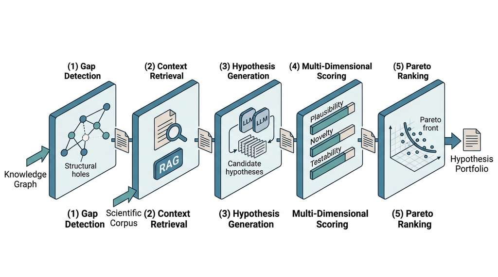
1. Gap Detection: Analyze the knowledge graph for structural holes (missing connections between otherwise well-connected communities) and embedding-space gaps (Section 39.1).
2. Context Retrieval: For each top-scoring gap, retrieve relevant passages from the scientific corpus using RAG (Chapter 37).
3. Hypothesis Generation: Use an LLM to generate candidate hypotheses grounded in the retrieved context (Section 39.2).
4. Multi-Dimensional Scoring: Score each hypothesis for plausibility, novelty, and testability (Section 39.2).
5. Pareto Ranking and Presentation: Rank hypotheses using Pareto dominance (explained below) and present results for human review.

Figure 39.11 shows how these five stages connect. Each stage consumes the typed output of the previous one and produces a new typed artifact, so any stage can be inspected, cached, or replaced independently.

Without a principled way to rank hypotheses across competing dimensions, scientists either drown in hundreds of unscored candidates or silently discard novel ideas because a single weighted formula penalizes anything unfamiliar. Pareto ranking solves this by surfacing every hypothesis that is optimal for some combination of priorities.

Pareto ranking is a multi-objective optimization technique that identifies solutions where no single objective can be improved without worsening another. It matters here because hypothesis evaluation involves inherently conflicting goals: a highly novel hypothesis is often less plausible, and vice versa. Collapsing these goals into a weighted sum forces an arbitrary choice of weights before seeing the results. The mechanism works by pairwise comparison. For each hypothesis, the algorithm counts how many others beat it on all three scoring dimensions simultaneously. Those that remain unbeaten form the "Pareto front" (rank 0). Use Pareto ranking whenever you have two or more scoring dimensions with no natural conversion rate between them. If your scores can be combined into a single number (for example, expected monetary value), a weighted sum suffices.

We implement this as a HypothesisGenerationPipeline class that orchestrates the full flow. In short: the pipeline turns a knowledge graph and a corpus into a portfolio of hypotheses ranked without forcing anyone to choose weights.

import networkx as nx
import numpy as np
import json
import logging
from dataclasses import dataclass, field, asdict
from datetime import datetime

import anthropic
from qdrant_client import QdrantClient
from qdrant_client.models import Distance, VectorParams, PointStruct
from sentence_transformers import SentenceTransformer

logger = logging.getLogger(__name__)


@dataclass
class ScoredHypothesis:
    """A hypothesis with all three scoring dimensions."""
    statement: str
    domain: str
    mechanism: str
    supporting_evidence: list[str]
    predictions: list[str]
    assumptions: list[str]
    source_gap: tuple[str, str]
    gap_score: float

    # Scoring dimensions
    plausibility: float = 0.0
    novelty: float = 0.0
    testability: float = 0.0

    # Testability details
    experiment_type: str = ""
    estimated_cost_usd: float = 0.0
    estimated_duration_days: int = 0

    # Pareto ranking
    pareto_rank: int = 0  # 0 = Pareto-optimal front
    dominated_by: int = 0  # Number of hypotheses that dominate this one

    # Metadata
    generated_at: str = field(
        default_factory=lambda: datetime.now().isoformat()
    )
    model_used: str = ""
    nearest_known_claims: list[str] = field(default_factory=list)


class HypothesisGenerationPipeline:
    """End-to-end pipeline for gap-based hypothesis generation.

    Orchestrates gap detection, context retrieval, LLM generation,
    multi-dimensional scoring, and Pareto ranking.
    """

    def __init__(
        self,
        knowledge_graph: nx.Graph,
        corpus_passages: list[str],
        known_claims: list[str],
        embedding_model: str = "all-MiniLM-L6-v2",
        llm_model: str = "claude-sonnet-4-20250514",
    ):
        self.G = knowledge_graph
        self.corpus = corpus_passages
        self.known_claims = known_claims
        self.llm_model = llm_model

        # Initialize embedding model and vector stores
        self.embedder = SentenceTransformer(embedding_model)
        self.qdrant = QdrantClient(":memory:")

        # Index corpus for retrieval
        self._index_corpus()
        # Index known claims for novelty scoring
        self._index_claims()

        # Anthropic client
        self.client = anthropic.Anthropic()

    def _index_corpus(self):
        """Index corpus passages in Qdrant for retrieval."""
        embeddings = self.embedder.encode(
            self.corpus, normalize_embeddings=True
        )
        dim = embeddings.shape[1]

        self.qdrant.create_collection(
            collection_name="corpus",
            vectors_config=VectorParams(
                size=dim, distance=Distance.COSINE
            ),
        )

        points = [
            PointStruct(id=i, vector=emb.tolist(),
                        payload={"text": text})
            for i, (text, emb) in enumerate(
                zip(self.corpus, embeddings)
            )
        ]
        self.qdrant.upsert(collection_name="corpus", points=points)

    def _index_claims(self):
        """Index known claims for novelty scoring."""
        embeddings = self.embedder.encode(
            self.known_claims, normalize_embeddings=True
        )
        dim = embeddings.shape[1]

        self.qdrant.create_collection(
            collection_name="claims",
            vectors_config=VectorParams(
                size=dim, distance=Distance.COSINE
            ),
        )

        points = [
            PointStruct(id=i, vector=emb.tolist(),
                        payload={"claim": claim})
            for i, (claim, emb) in enumerate(
                zip(self.known_claims, embeddings)
            )
        ]
        self.qdrant.upsert(collection_name="claims", points=points)

    def run(
        self,
        max_gaps: int = 20,
        hypotheses_per_gap: int = 3,
        min_gap_score: float = 0.1,
    ) -> list[ScoredHypothesis]:
        """Execute the full hypothesis generation pipeline.

        Args:
            max_gaps: Maximum number of gaps to process.
            hypotheses_per_gap: Hypotheses to generate per gap.
            min_gap_score: Minimum gap score threshold.

        Returns:
            Pareto-ranked list of scored hypotheses.
        """
        # Stage 1: Gap Detection
        logger.info("Stage 1: Detecting knowledge gaps...")
        gaps = self._detect_gaps(max_gaps, min_gap_score)
        logger.info(f"Found {len(gaps)} gaps above threshold.")

        # Stage 2-3: Context Retrieval + Hypothesis Generation
        all_hypotheses = []
        for entity_a, entity_b, gap_score in gaps:
            logger.info(
                f"Processing gap: {entity_a} <-> {entity_b} "
                f"(score={gap_score:.3f})"
            )

            # Retrieve context
            context = self._retrieve_context(entity_a, entity_b)

            # Generate hypotheses
            hypotheses = self._generate_hypotheses(
                entity_a, entity_b, context,
                n=hypotheses_per_gap, gap_score=gap_score,
            )
            all_hypotheses.extend(hypotheses)

        logger.info(
            f"Generated {len(all_hypotheses)} raw hypotheses."
        )

        # Stage 4: Multi-Dimensional Scoring
        logger.info("Stage 4: Scoring hypotheses...")
        scored = self._score_all(all_hypotheses)

        # Stage 5: Pareto Ranking
        logger.info("Stage 5: Computing Pareto ranking...")
        ranked = self._pareto_rank(scored)

        logger.info(
            f"Pipeline complete. "
            f"{sum(1 for h in ranked if h.pareto_rank == 0)} "
            f"hypotheses on the Pareto front."
        )
        return ranked

    def _detect_gaps(
        self,
        max_gaps: int,
        min_score: float,
    ) -> list[tuple[str, str, float]]:
        """Detect structural holes in the knowledge graph."""
        # Louvain community detection partitions the graph into
        # densely connected groups; gaps between communities are
        # the most promising sites for novel hypotheses.
        communities = nx.community.louvain_communities(
            self.G, seed=42
        )
        node_to_comm = {}
        for idx, comm in enumerate(communities):
            for node in comm:
                node_to_comm[node] = idx

        candidates = [n for n, d in self.G.degree() if d >= 2]
        path_lengths = dict(
            nx.all_pairs_shortest_path_length(self.G, cutoff=4)
        )

        from itertools import combinations
        gaps = []
        for u, v in combinations(candidates, 2):
            if self.G.has_edge(u, v):
                continue
            dist = path_lengths.get(u, {}).get(v)
            if dist is None or dist > 4:
                continue
            if node_to_comm.get(u) == node_to_comm.get(v):
                continue

            n_u = set(self.G.neighbors(u))
            n_v = set(self.G.neighbors(v))
            union = n_u | n_v
            if not union:
                continue
            jaccard_comp = 1.0 - len(n_u & n_v) / len(union)
            score = (len(n_u) * len(n_v) / dist**2) * jaccard_comp

            if score >= min_score:
                gaps.append((u, v, score))

        gaps.sort(key=lambda x: x[2], reverse=True)
        return gaps[:max_gaps]

    def _retrieve_context(
        self,
        entity_a: str,
        entity_b: str,
        top_k: int = 8,
    ) -> list[str]:
        """Retrieve relevant corpus passages for a gap."""
        query = f"{entity_a} {entity_b} relationship mechanism"
        q_emb = self.embedder.encode(
            [query], normalize_embeddings=True
        )[0]

        results = self.qdrant.search(
            collection_name="corpus",
            query_vector=q_emb.tolist(),
            limit=top_k,
        )
        return [r.payload["text"] for r in results]

    def _generate_hypotheses(
        self,
        entity_a: str,
        entity_b: str,
        context: list[str],
        n: int = 3,
        gap_score: float = 0.0,
    ) -> list[ScoredHypothesis]:
        """Generate hypotheses for a gap using Claude."""
        context_block = "\n\n".join(
            f"[{i+1}]: {p}" for i, p in enumerate(context)
        )

        prompt = f"""Knowledge gap between "{entity_a}" and "{entity_b}".

Literature context:
{context_block}

Generate {n} distinct, testable hypotheses about how {entity_a}
and {entity_b} might be related. Each hypothesis must propose a
DIFFERENT mechanism.

Return a JSON array where each element has:
- "statement": one-sentence hypothesis
- "domain": scientific domain
- "mechanism": 2-3 sentence causal explanation
- "supporting_evidence": list of evidence points from the context
- "predictions": list of specific, falsifiable predictions
- "assumptions": list of assumptions that must hold"""

        response = self.client.messages.create(
            model=self.llm_model,
            max_tokens=4096,
            system="You are a scientific hypothesis generator. "
                   "Return ONLY valid JSON. Be specific and precise.",
            messages=[{"role": "user", "content": prompt}],
        )

        text = response.content[0].text
        if "```json" in text:
            text = text.split("```json")[1].split("```")[0]
        elif "```" in text:
            text = text.split("```")[1].split("```")[0]

        try:
            raw = json.loads(text)
        except json.JSONDecodeError:
            logger.warning(
                f"Failed to parse LLM output for gap "
                f"{entity_a}<->{entity_b}"
            )
            return []

        if isinstance(raw, dict):
            raw = [raw]

        hypotheses = []
        for h in raw:
            hypotheses.append(ScoredHypothesis(
                statement=h.get("statement", ""),
                domain=h.get("domain", "unknown"),
                mechanism=h.get("mechanism", ""),
                supporting_evidence=h.get("supporting_evidence", []),
                predictions=h.get("predictions", []),
                assumptions=h.get("assumptions", []),
                source_gap=(entity_a, entity_b),
                gap_score=gap_score,
                model_used=self.llm_model,
            ))
        return hypotheses

    def _score_all(
        self,
        hypotheses: list[ScoredHypothesis],
    ) -> list[ScoredHypothesis]:
        """Score all hypotheses on three dimensions."""
        for h in hypotheses:
            # Plausibility: semantic consistency with evidence
            h.plausibility = self._score_plausibility(h)
            # Novelty: embedding distance from known claims
            novelty_result = self._score_novelty(h)
            h.novelty = novelty_result["score"]
            h.nearest_known_claims = novelty_result["nearest"]
            # Testability: experiment cost estimation
            h.testability = self._score_testability(h)

        return hypotheses

    def _score_plausibility(self, h: ScoredHypothesis) -> float:
        """Plausibility as semantic consistency with evidence."""
        if not h.supporting_evidence:
            return 0.3  # Low default for unsupported hypotheses

        all_texts = [h.statement] + h.supporting_evidence
        embeddings = self.embedder.encode(
            all_texts, normalize_embeddings=True
        )
        h_emb = embeddings[0]
        e_embs = embeddings[1:]
        similarities = e_embs @ h_emb

        # Weight by gap score (higher gap score = stronger prior)
        base = float(np.mean(similarities))
        prior_boost = h.gap_score / (h.gap_score + 1.0)
        return float(np.clip(
            0.7 * base + 0.3 * prior_boost, 0.0, 1.0
        ))

    def _score_novelty(
        self, h: ScoredHypothesis,
    ) -> dict:
        """Novelty as distance from nearest known claim."""
        h_emb = self.embedder.encode(
            [h.statement], normalize_embeddings=True
        )[0]

        results = self.qdrant.search(
            collection_name="claims",
            query_vector=h_emb.tolist(),
            limit=3,
        )

        if not results:
            return {"score": 1.0, "nearest": []}

        max_sim = results[0].score
        nearest = [r.payload["claim"] for r in results]
        return {
            "score": float(1.0 - max_sim),
            "nearest": nearest,
        }

    def _score_testability(self, h: ScoredHypothesis) -> float:
        """Testability based on LLM experiment cost estimation."""
        import math

        prompt = f"""Briefly assess the testability of this hypothesis.
Hypothesis: {h.statement}
Predictions: {json.dumps(h.predictions[:3])}

Choose the cheapest experiment type that could test this:
- computational_simulation ($10/run, 1 day)
- spectroscopy_measurement ($200/run, 1 day)
- genomics_sequencing ($300/run, 7 days)
- cell_culture_assay ($500/run, 14 days)
- materials_synthesis ($1000/run, 7 days)
- animal_model ($5000/run, 90 days)
- clinical_trial_phase1 ($1000000/run, 365 days)

Return JSON: {{"experiment_type": "...", "runs_needed": N}}"""

        try:
            response = self.client.messages.create(
                model=self.llm_model,
                max_tokens=256,
                messages=[{"role": "user", "content": prompt}],
            )
            text = response.content[0].text
            if "```json" in text:
                text = text.split("```json")[1].split("```")[0]
            elif "```" in text:
                text = text.split("```")[1].split("```")[0]

            data = json.loads(text)
            exp_type = data.get(
                "experiment_type", "cell_culture_assay"
            )
            runs = data.get("runs_needed", 10)

            cost_table = {
                "computational_simulation": 10,
                "spectroscopy_measurement": 200,
                "genomics_sequencing": 300,
                "cell_culture_assay": 500,
                "materials_synthesis": 1000,
                "animal_model": 5000,
                "clinical_trial_phase1": 1_000_000,
            }
            cost_per = cost_table.get(exp_type, 500)
            total = cost_per * runs
            h.experiment_type = exp_type
            h.estimated_cost_usd = total

            # Log-scale normalization: $10 -> 1.0, $10M -> 0.0
            score = 1.0 - math.log10(total + 1) / 7.0
            return float(np.clip(score, 0.0, 1.0))

        except (json.JSONDecodeError, KeyError):
            h.experiment_type = "unknown"
            h.estimated_cost_usd = 0
            return 0.5  # Default middle score on parse failure

    def _pareto_rank(
        self,
        hypotheses: list[ScoredHypothesis],
    ) -> list[ScoredHypothesis]:
        """Assign Pareto ranks based on three scoring dimensions.

        A hypothesis H1 dominates H2 if H1 is at least as good
        as H2 on ALL three dimensions and strictly better on at
        least one. The Pareto front (rank 0) consists of
        non-dominated hypotheses.
        """
        n = len(hypotheses)
        scores = np.array([
            [h.plausibility, h.novelty, h.testability]
            for h in hypotheses
        ])

        # Count dominations
        for i in range(n):
            count = 0
            for j in range(n):
                if i == j:
                    continue
                # j dominates i if j >= i on all and j > i on some
                if (np.all(scores[j] >= scores[i])
                        and np.any(scores[j] > scores[i])):
                    count += 1
            hypotheses[i].dominated_by = count
            hypotheses[i].pareto_rank = count  # Rank = # dominators

        # Sort by Pareto rank, then by sum of scores within rank
        hypotheses.sort(
            key=lambda h: (
                h.pareto_rank,
                -(h.plausibility + h.novelty + h.testability),
            )
        )
        return hypotheses

2. Running the Pipeline

The following example shows how the full pipeline performs on real scientific data.

Let us run the complete pipeline on a concrete example: hypothesis generation for a biomedical knowledge graph focused on neurodegeneration. We construct a knowledge graph from known gene-disease and drug-target relations, provide a corpus of relevant abstracts, and examine the output:

import networkx as nx

# Construct a biomedical knowledge graph
G = nx.Graph()

# Gene-disease relations (neurodegenerative focus)
gene_disease = [
    ("APP", "alzheimers"), ("PSEN1", "alzheimers"),
    ("MAPT", "alzheimers"), ("MAPT", "ftd"),
    ("SNCA", "parkinsons"), ("LRRK2", "parkinsons"),
    ("GBA", "parkinsons"), ("GBA", "gaucher"),
    ("SOD1", "als"), ("C9orf72", "als"), ("C9orf72", "ftd"),
    ("HTT", "huntingtons"),
    ("TREM2", "alzheimers"), ("TREM2", "neuroinflammation"),
    ("APOE", "alzheimers"), ("APOE", "cardiovascular"),
]

# Gene-gene interactions
gene_gene = [
    ("APP", "PSEN1"), ("APP", "MAPT"), ("SNCA", "LRRK2"),
    ("SNCA", "GBA"), ("SOD1", "C9orf72"),
    ("TREM2", "APOE"), ("LRRK2", "GBA"),
]

# Drug-target relations
drug_target = [
    ("lecanemab", "APP"), ("aducanumab", "APP"),
    ("levodopa", "dopamine_system"), ("SNCA", "dopamine_system"),
    ("riluzole", "glutamate_system"), ("SOD1", "glutamate_system"),
    ("donepezil", "acetylcholine_system"),
    ("acetylcholine_system", "alzheimers"),
]

# Pathway connections
pathways = [
    ("neuroinflammation", "alzheimers"),
    ("neuroinflammation", "parkinsons"),
    ("neuroinflammation", "als"),
    ("autophagy", "parkinsons"), ("GBA", "autophagy"),
    ("LRRK2", "autophagy"),
    ("mitochondria", "parkinsons"), ("mitochondria", "als"),
    ("protein_aggregation", "alzheimers"),
    ("protein_aggregation", "parkinsons"),
    ("protein_aggregation", "huntingtons"),
]

G.add_edges_from(
    gene_disease + gene_gene + drug_target + pathways
)

# Sample corpus passages (in production, retrieved from PubMed)
corpus = [
    "TREM2 variants increase Alzheimer's risk through impaired "
    "microglial clearance of amyloid plaques.",
    "GBA mutations cause lysosomal dysfunction, leading to "
    "alpha-synuclein accumulation in Parkinson's disease.",
    "Neuroinflammation is a shared pathological feature across "
    "Alzheimer's, Parkinson's, and ALS.",
    "LRRK2 kinase activity regulates autophagy flux and is "
    "elevated in Parkinson's disease brain tissue.",
    "C9orf72 repeat expansions cause both ALS and FTD through "
    "RNA toxicity and dipeptide repeat proteins.",
    "APOE4 impairs blood-brain barrier integrity and promotes "
    "neuroinflammation independent of amyloid pathology.",
    "Mitochondrial dysfunction is an early feature of both "
    "Parkinson's disease and ALS pathogenesis.",
    "The autophagy-lysosome pathway is a convergence point for "
    "multiple neurodegenerative disease mechanisms.",
    "Protein aggregation, once initiated, can spread between "
    "cells in a prion-like manner across brain regions.",
    "Microglial activation states shift from neuroprotective to "
    "neurotoxic during disease progression.",
]

# Known claims (for novelty scoring)
known_claims = [
    "TREM2 loss of function increases Alzheimer's disease risk.",
    "GBA mutations are the most common genetic risk factor for "
    "Parkinson's disease.",
    "Lecanemab reduces amyloid plaques in Alzheimer's patients.",
    "Neuroinflammation contributes to neurodegeneration.",
    "LRRK2 G2019S is the most common genetic cause of familial "
    "Parkinson's disease.",
    "Alpha-synuclein aggregation is a hallmark of Parkinson's.",
    "APOE4 is the strongest genetic risk factor for late-onset "
    "Alzheimer's disease.",
]

# Run the pipeline
pipeline = HypothesisGenerationPipeline(
    knowledge_graph=G,
    corpus_passages=corpus,
    known_claims=known_claims,
    llm_model="claude-sonnet-4-20250514",
)

results = pipeline.run(
    max_gaps=10,
    hypotheses_per_gap=3,
    min_gap_score=0.1,
)

# Display Pareto-optimal hypotheses
print("=" * 60)
print("PARETO-OPTIMAL HYPOTHESES (Rank 0)")
print("=" * 60)
for h in results:
    if h.pareto_rank > 0:
        break
    print(f"\n--- {h.source_gap[0]} <-> {h.source_gap[1]} ---")
    print(f"Statement: {h.statement}")
    print(f"Plausibility: {h.plausibility:.3f}")
    print(f"Novelty:      {h.novelty:.3f}")
    print(f"Testability:  {h.testability:.3f}")
    print(f"Experiment:   {h.experiment_type}")
    print(f"Est. cost:    ${h.estimated_cost_usd:,.0f}")
    if h.nearest_known_claims:
        print(f"Nearest claim: {h.nearest_known_claims[0][:80]}...")

3. Visualization and Export

A ranked list of hypotheses is useful, but a structured export makes the portfolio portable and machine-readable. The following utility writes the scored hypotheses as JSON files that downstream tools (visualization scripts, research agents, or the Discovery Workbench) can consume directly. The lab exercise at the end of this section walks through building an interactive 3D scatter plot from this exported data:

import json
from pathlib import Path
from dataclasses import asdict


def export_hypothesis_portfolio(
    hypotheses: list[ScoredHypothesis],
    output_dir: str = "hypothesis_portfolio",
) -> Path:
    """Export scored hypotheses as a structured JSON portfolio.

    Creates a directory with:
    - portfolio.json: Full scored hypothesis data
    - summary.json: Pareto front summary for quick review
    - per-hypothesis detail files
    """
    out = Path(output_dir)
    out.mkdir(parents=True, exist_ok=True)

    # Full portfolio
    portfolio = {
        "generated_at": datetime.now().isoformat(),
        "total_hypotheses": len(hypotheses),
        "pareto_front_size": sum(
            1 for h in hypotheses if h.pareto_rank == 0
        ),
        "hypotheses": [
            {
                "rank": i,
                "pareto_rank": h.pareto_rank,
                "statement": h.statement,
                "domain": h.domain,
                "mechanism": h.mechanism,
                "source_gap": list(h.source_gap),
                "scores": {
                    "plausibility": round(h.plausibility, 4),
                    "novelty": round(h.novelty, 4),
                    "testability": round(h.testability, 4),
                },
                "experiment": {
                    "type": h.experiment_type,
                    "estimated_cost_usd": h.estimated_cost_usd,
                    "estimated_duration_days": h.estimated_duration_days,
                },
                "predictions": h.predictions,
                "assumptions": h.assumptions,
                "supporting_evidence": h.supporting_evidence,
                "nearest_known_claims": h.nearest_known_claims,
            }
            for i, h in enumerate(hypotheses)
        ],
    }

    portfolio_path = out / "portfolio.json"
    portfolio_path.write_text(json.dumps(portfolio, indent=2))

    # Summary of Pareto front for quick review
    pareto_front = [
        {
            "statement": h.statement,
            "scores": f"P={h.plausibility:.2f} "
                      f"N={h.novelty:.2f} "
                      f"T={h.testability:.2f}",
            "experiment": h.experiment_type,
            "cost": f"${h.estimated_cost_usd:,.0f}",
        }
        for h in hypotheses if h.pareto_rank == 0
    ]

    summary_path = out / "summary.json"
    summary_path.write_text(json.dumps(pareto_front, indent=2))

    logger.info(
        f"Exported {len(hypotheses)} hypotheses to {out}. "
        f"Pareto front: {len(pareto_front)} hypotheses."
    )
    return out

4. Interpreting the Scoring Landscape

The structured JSON portfolio is portable, but its real value emerges when scientists read the three scoring dimensions as a diagnostic of each hypothesis.

The three scoring dimensions create a natural taxonomy of hypothesis types. Understanding this taxonomy helps scientists navigate the portfolio:

Three Hypothesis Archetypes

High plausibility, low novelty, high testability: incremental hypotheses. These propose well-grounded extensions of existing knowledge that can be tested cheaply. They are the "safe bets" of the portfolio, likely to yield positive results but unlikely to produce surprising discoveries. Example: "LRRK2 kinase inhibitors reduce neuroinflammation in Parkinson's disease models" (plausible because both LRRK2 and neuroinflammation are established Parkinson's factors; low novelty because the connection is already suspected; testable with standard cell culture assays).

Moderate plausibility, high novelty, moderate testability: frontier hypotheses. These propose connections that are consistent with some evidence but have not been explored. They are the highest-value targets for discovery. Example: "GBA lysosomal dysfunction contributes to Alzheimer's pathology through impaired TREM2-mediated amyloid clearance" (moderately plausible because GBA and TREM2 are both linked to neurodegeneration through different pathways; novel because their interaction is unstudied; testable with cell culture but requiring specialized assays).

Low plausibility, high novelty, low testability: speculative hypotheses. These propose entirely new connections with limited supporting evidence. Most will turn out to be wrong, but the few that survive testing could be transformative. A research group pursuing these hypotheses needs a high tolerance for failure and the resources to invest in exploratory experiments.

5. Integration with the Discovery Workbench

The hypothesis generation pipeline produces structured output (the JSON portfolio) that plugs directly into the Discovery Workbench architecture from Chapter 6. The integration points are:

• Knowledge graph input: the pipeline consumes graphs produced by the knowledge graph construction pipeline of Chapter 38.
• Corpus input: passages come from the RAG retrieval system of Chapter 37, which indexes the literature mined in Chapter 36.
• Hypothesis output: the scored portfolio feeds into the research agents of Chapter 40, which can autonomously pursue top-ranked hypotheses.
• Validation loop: hypotheses that survive research agent investigation enter the claim validation pipeline of Chapter 41.

class DiscoveryWorkbenchIntegration:
    """Connect the hypothesis pipeline to the Discovery Workbench.

    Provides methods to load knowledge graphs and corpora from
    the Workbench's data stores, run the pipeline, and publish
    results back to the Workbench for downstream consumption
    by research agents and claim validators.
    """

    def __init__(self, workbench_config: dict):
        self.config = workbench_config
        self.pipeline = None

    def load_from_workbench(
        self,
        kg_collection: str = "knowledge_graph",
        corpus_collection: str = "literature_corpus",
        claims_collection: str = "validated_claims",
    ):
        """Load pipeline inputs from Workbench data stores."""
        # Load knowledge graph from the KG store (Chapter 38)
        G = self._load_knowledge_graph(kg_collection)

        # Load corpus from the RAG index (Chapter 37)
        corpus = self._load_corpus(corpus_collection)

        # Load known claims from the claim validator (Chapter 41)
        claims = self._load_claims(claims_collection)

        self.pipeline = HypothesisGenerationPipeline(
            knowledge_graph=G,
            corpus_passages=corpus,
            known_claims=claims,
        )
        return self

    def run_and_publish(
        self,
        max_gaps: int = 20,
        hypotheses_per_gap: int = 3,
    ) -> list[ScoredHypothesis]:
        """Run the pipeline and publish results to the Workbench."""
        results = self.pipeline.run(
            max_gaps=max_gaps,
            hypotheses_per_gap=hypotheses_per_gap,
        )

        # Publish to Workbench hypothesis store
        self._publish_hypotheses(results)

        # Notify research agents of new high-priority hypotheses
        pareto_front = [h for h in results if h.pareto_rank == 0]
        self._notify_research_agents(pareto_front)

        return results

    def _load_knowledge_graph(self, collection: str) -> nx.Graph:
        """Load KG from Workbench. Implementation depends on
        the specific Workbench backend (Neo4j, NetworkX, etc.)."""
        # Placeholder: in production, this reads from the
        # Chapter 38 knowledge graph store
        return nx.Graph()

    def _load_corpus(self, collection: str) -> list[str]:
        """Load corpus from the RAG index."""
        return []

    def _load_claims(self, collection: str) -> list[str]:
        """Load validated claims from the claim store."""
        return []

    def _publish_hypotheses(
        self, hypotheses: list[ScoredHypothesis]
    ):
        """Write scored hypotheses to the Workbench store."""
        logger.info(
            f"Published {len(hypotheses)} hypotheses "
            f"to Workbench."
        )

    def _notify_research_agents(
        self, pareto_front: list[ScoredHypothesis]
    ):
        """Notify research agents (Chapter 40) of new
        high-priority hypotheses for autonomous investigation."""
        logger.info(
            f"Notified agents of {len(pareto_front)} "
            f"Pareto-optimal hypotheses."
        )

6. Cost Management and Caching

Once the pipeline is wired into the Workbench and running on production-scale knowledge graphs, the dominant practical concern shifts from correctness to cost.

The pipeline makes multiple LLM calls per gap (generation + testability assessment), which can become expensive at scale. For a knowledge graph with 20 gaps and 3 hypotheses per gap, the pipeline makes approximately 80 API calls. At typical mid-2025 rates, this costs roughly \$2 to \$5 per pipeline run. (That is sixty testable scientific hypotheses for the price of a latte; the bottleneck has shifted entirely from generation to evaluation.) For daily runs on a large knowledge graph (200 gaps), the monthly cost can reach \$500 to \$1,500.

Two strategies keep costs manageable. First, cache LLM responses keyed by the prompt hash. When the pipeline re-analyzes the same gap with the same context (common during incremental knowledge graph updates), it reuses the cached response instead of calling the API again. Second, use a tiered model strategy. Route testability assessments to cheaper models (Claude Haiku or GPT-4o-mini), since the output is a short JSON classification. Reserve more capable models (Claude Sonnet or GPT-4o) for hypothesis generation, where output quality matters more:

import hashlib
import json
from pathlib import Path


class LLMCache:
    """Simple disk-based cache for LLM responses."""

    def __init__(self, cache_dir: str = ".hypothesis_cache"):
        self.cache_dir = Path(cache_dir)
        self.cache_dir.mkdir(parents=True, exist_ok=True)

    def _key(self, prompt: str, model: str) -> str:
        content = f"{model}:{prompt}"
        return hashlib.sha256(content.encode()).hexdigest()[:16]

    def get(self, prompt: str, model: str) -> str | None:
        path = self.cache_dir / f"{self._key(prompt, model)}.json"
        if path.exists():
            data = json.loads(path.read_text())
            return data["response"]
        return None

    def put(self, prompt: str, model: str, response: str):
        path = self.cache_dir / f"{self._key(prompt, model)}.json"
        data = {
            "prompt_hash": self._key(prompt, model),
            "model": model,
            "response": response,
        }
        path.write_text(json.dumps(data))


# Usage in the pipeline:
# cache = LLMCache()
# cached = cache.get(prompt, model)
# if cached:
#     text = cached
# else:
#     response = client.messages.create(...)
#     text = response.content[0].text
#     cache.put(prompt, model, text)

Exercises

1. (Conceptual) The Pareto ranking approach treats plausibility, novelty, and testability as equally important dimensions. But a pharmaceutical company might weight testability heavily (they need U.S. Food and Drug Administration (FDA)-approvable experiments), while a theoretical physics group might weight novelty heavily (incremental results are less publishable). Design a user interface that lets a scientist express their preferences as constraints ("novelty must be at least 0.4") or weights, and show how this changes the effective Pareto front. How does the front shrink or expand as constraints tighten?
2. (Coding) Extend the pipeline with a "hypothesis diversity" filter: after Pareto ranking, ensure that the top-K hypotheses span at least 3 different source gaps and at least 2 different experiment types. Implement this as a greedy diversification step that maximizes the minimum pairwise embedding distance among selected hypotheses. Compare the diversified portfolio against the raw Pareto ranking on a knowledge graph of your choice.
3. (Project) Build a complete hypothesis generation system for a scientific domain you are familiar with. Construct a knowledge graph from at least 100 papers (using techniques from Chapters 36 and 38), run the pipeline, and evaluate the top 5 hypotheses by searching the literature for evidence that either supports or contradicts them. Write a one-page assessment of the pipeline's output quality, including false positives (implausible hypotheses ranked highly) and false negatives (important gaps the pipeline missed).