"I gave each agent three simple rules and stepped back. By iteration 500, they had invented traffic jams, housing segregation, and a stock market. I had only asked them to move toward food."
A Mesa Model With Emergent Regret
A computational experiment is a controlled, reproducible run of a simulator that tests a specific hypothesis about a system's behavior. Unlike physical experiments, computational experiments let you vary one parameter at a time with perfect precision, replay the same random seed to isolate stochastic effects, and observe internal states that no instrument can measure. This section introduces two simulation paradigms: agent-based modeling for emergent phenomena and discrete-event simulation for process-driven systems. Both share a common architecture of entities, rules, time advancement, and data collection that we formalize before writing any code.
1. Why Simulate?
What if you could rewind a pandemic to the day before a lockdown decision, change one policy parameter, and watch twelve months of consequences unfold in under a minute? Among the discovery paradigms we introduced in Chapter 5, simulation is the one that grants this power: theory gives you equations, data gives you correlations, but simulation gives you mechanistic narratives. You encode your hypothesized mechanism as executable rules, run the system forward, and compare the emergent behavior to observations. When the simulation matches reality, every rule in the code becomes a candidate explanation. When it fails, the mismatch tells you which rule is wrong.
To harness that power systematically, we need a precise vocabulary for what a computational experiment involves and when simulation is the right tool.
What. A computational experiment is the execution of a simulator under controlled conditions (fixed parameters, specified initial state, recorded random seed) with systematic data collection for subsequent analysis.
Why. Three reasons dominate scientific simulation. First, inaccessibility: no physical experiment can probe planetary formation, pandemic spread, or protein folding at atomic resolution. Second, cost: a drug trial costs billions; a pharmacokinetics simulation costs compute cycles. Third, interpretability: a simulation lets you inspect every intermediate state, pause time, and ask counterfactual questions ("What if this receptor were blocked?") that no physical experiment supports.
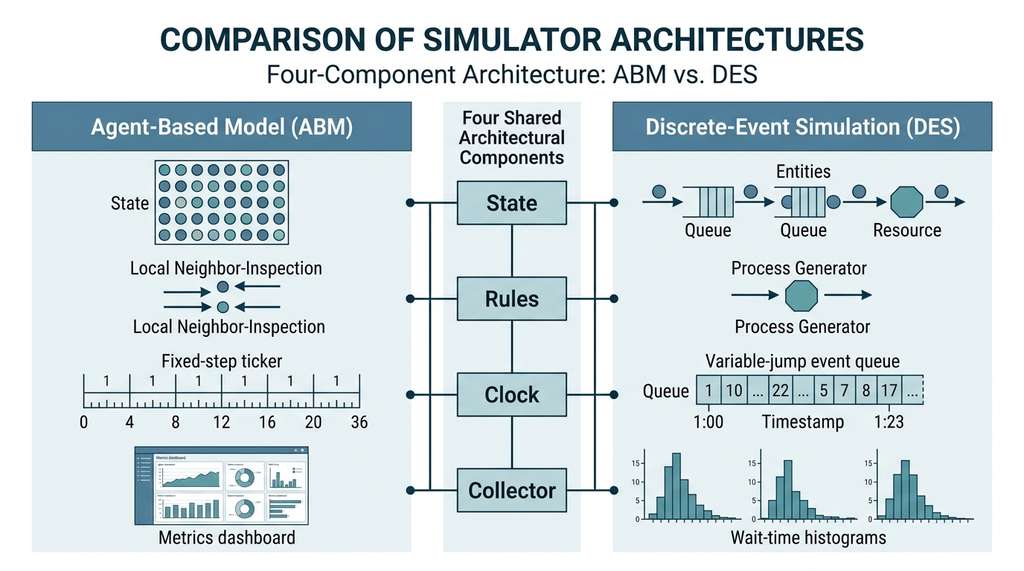
How. Every simulator shares four architectural components: (1) a state that describes the system at a given time, (2) rules that update the state, (3) a clock that advances time, and (4) a collector that records observables. The differences between paradigms lie in how these components are structured. Figure 43.1 illustrates how these four components connect in the simulation loop. Figure 43.1.1 illustrates simulator architecture: state-rules-clock-collector with ABM vs DES instantiation.
When. Simulate when you have a mechanistic hypothesis to test, when physical experiments are infeasible or unethical, when you need to generate synthetic training data for machine learning models, or when you want to explore the consequences of interventions before committing resources.
A simulator is a theory you can run. Unlike a mathematical model that you solve analytically, a simulator lets you encode complex, heterogeneous, stochastic mechanisms that have no closed-form solution. The Gillespie algorithm (Section 43.2) makes this concrete: you write down reaction rates, and the algorithm produces exact sample paths of the stochastic process, no differential equations required. This "executable theory" perspective connects simulation to the knowledge representation ideas from Chapter 3: your code is your ontology.
2. Agent-Based Models
In 2020, epidemiologists needed to compare dozens of lockdown strategies for COVID-19 before any could be tested on real populations; the cost of choosing wrong was measured in thousands of lives. Agent-based models made those comparisons possible in days rather than months, because they can encode millions of heterogeneous individuals following realistic behavioral rules and reveal collective outcomes that no equation-based model can predict.
Agent-based models (ABMs) represent a system as a collection of autonomous agents that interact according to local rules. No agent sees the whole system. No central controller dictates global behavior. Instead, macroscopic phenomena emerge from microscopic interactions, exactly as traffic jams emerge from individual driving decisions, or as segregation patterns emerge from mild individual preferences about neighbors.
An agent-based model places many independent software entities ("agents") in a shared environment. Each agent follows its own behavioral rules, and their interactions produce collective dynamics that no single agent was programmed to create. ABMs let scientists study emergence, where emergence is the appearance of complex macro-level patterns (market crashes, epidemic waves, ecosystem shifts) from simple micro-level interactions that resist prediction from any individual component alone. The mechanism works as follows: at each time step, every agent perceives its local neighborhood, applies its decision rules, and updates its state. The framework then collects system-wide statistics, tracking how micro-behavior aggregates into macro-patterns. Choose an ABM over equation-based models when your system contains heterogeneous actors with adaptive behavior, when spatial structure or network topology matters, or when aggregate dynamics depend on individual-level variability that a mean-field equation (an approximation that replaces all individual interactions with a single average effect) would average away.
The canonical example is Schelling's segregation model (1971). Agents of two types occupy cells on a grid. Each agent has a tolerance threshold: if fewer than, say, 30% of its neighbors are the same type, it moves to a random empty cell. Despite this mild preference, the system tends to self-organize into highly segregated clusters within tens of steps. The emergent macro-pattern (segregation) is far more extreme than any individual agent's preference would predict.
Mental Model
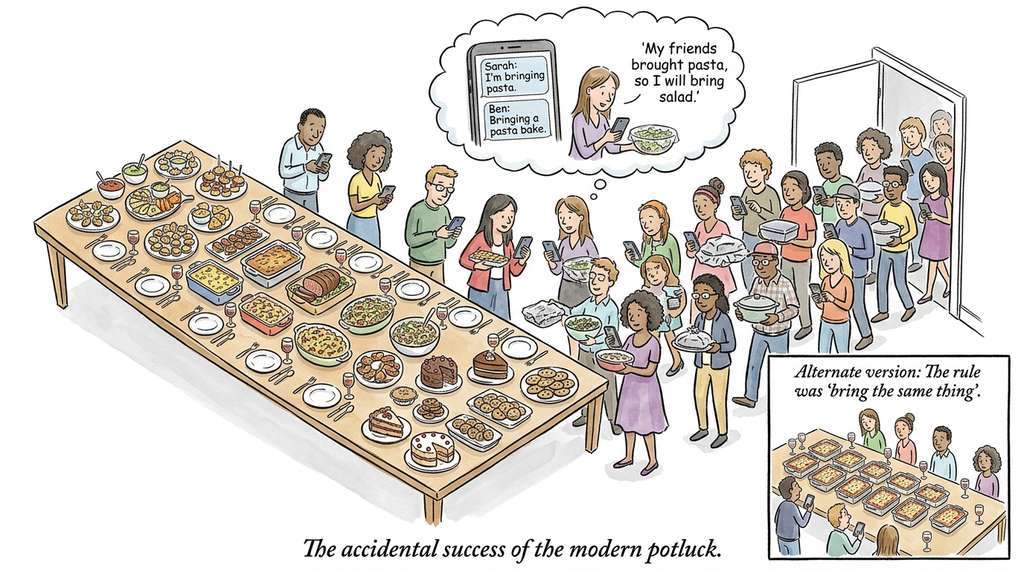
Emergence in an ABM works like a potluck dinner. Each guest (agent) follows one personal rule: "bring a dish that complements what my two closest friends are bringing." Nobody plans the full menu. Yet when thirty guests arrive, the table reliably ends up with a balanced spread of appetizers, mains, and desserts, a macro-pattern no individual orchestrated. If you change the rule slightly ("bring the same dish as your friends"), everyone shows up with lasagna. The analogy maps precisely: agents have local information and simple rules, coordination happens through indirect feedback (seeing neighbors' choices), and the collective outcome is qualitatively different from, and often surprising given, any single agent's intention. When a Schelling agent relocates because too few neighbors match, that move changes the neighborhood composition for everyone nearby, triggering a cascade, just as one guest switching from salad to pasta reshuffles the signals for the whole friend group.
2.1 The Mesa Framework
Mesa is a Python framework for agent-based modeling that provides the scaffolding every ABM needs: an agent class, a model class, a scheduler, a spatial grid, and a data collector. Building Schelling's model from scratch reveals the architecture. In short: encode your agents' local rules, hand the rest to the framework, and let emergence do the explaining.
import mesa
import numpy as np


class SchellingAgent(mesa.Agent):
    """An agent with a type and a happiness threshold."""

    def __init__(self, model, agent_type, homophily):
        super().__init__(model)
        self.type = agent_type
        self.homophily = homophily  # fraction of same-type neighbors desired

    def step(self):
        neighbors = self.model.grid.get_neighbors(
            self.pos, moore=True, include_center=False
        )
        if len(neighbors) == 0:
            return

        same_type = sum(1 for n in neighbors if n.type == self.type)
        fraction_same = same_type / len(neighbors)

        if fraction_same < self.homophily:
            # Unhappy: move to a random empty cell
            self.model.grid.move_to_empty(self)
        else:
            self.model.happy += 1


class SchellingModel(mesa.Model):
    """Schelling segregation model."""

    def __init__(self, width=20, height=20, density=0.8,
                 minority_fraction=0.5, homophily=0.3, seed=None):
        super().__init__(seed=seed)
        self.grid = mesa.space.SingleGrid(width, height, torus=True)
        self.happy = 0

        # Place agents on the grid
        for cell in self.grid.coord_iter():
            x, y = cell[1], cell[2]
            if self.random.random() < density:
                agent_type = (
                    0 if self.random.random() < minority_fraction else 1
                )
                agent = SchellingAgent(self, agent_type, homophily)
                self.grid.place_agent(agent, (x, y))

        # Data collector records segregation metrics each step
        self.datacollector = mesa.DataCollector(
            model_reporters={
                "happy_fraction": lambda m: (
                    m.happy / len(m.agents) if m.agents else 0
                ),
                "segregation_index": self._segregation_index,
            }
        )

    def _segregation_index(self):
        """Average fraction of same-type neighbors across all agents."""
        fractions = []
        for agent in self.agents:
            neighbors = self.grid.get_neighbors(
                agent.pos, moore=True, include_center=False
            )
            if neighbors:
                same = sum(1 for n in neighbors if n.type == agent.type)
                fractions.append(same / len(neighbors))
        return np.mean(fractions) if fractions else 0.0

    def step(self):
        self.happy = 0
        self.agents.shuffle_do("step")
        self.datacollector.collect(self)


# Run the model
model = SchellingModel(width=20, height=20, homophily=0.3, seed=42)
for _ in range(50):
    model.step()

results = model.datacollector.get_model_dataframe()
print(f"Final segregation index: {results['segregation_index'].iloc[-1]:.3f}")
print(f"Final happy fraction: {results['happy_fraction'].iloc[-1]:.3f}")moore=True means each cell considers all eight surrounding cells, including diagonals) and a toroidal grid (where torus=True wraps the edges so agents on one border neighbor agents on the opposite border). The DataCollector records the segregation index at each step, enabling analysis of how micro-preferences produce macro-segregation.The output reveals the signature Schelling phenomenon: with a homophily threshold of just 0.3, the segregation index climbs well above 0.7, meaning agents who require only 30% similarity end up in neighborhoods that are over 70% homogeneous. Agents who would happily live in a mixed neighborhood collectively produce a segregated city.
Public health agencies use agent-based models to evaluate intervention strategies before implementing them. An ABM of disease spread assigns each agent a health state (susceptible, infected, recovered), a contact network, and behavioral rules (mask wearing, social distancing). By running thousands of simulations with different intervention timings and coverages, analysts can estimate the distribution of outcomes for each policy option. The UK's London School of Hygiene & Tropical Medicine (LSHTM) model for COVID-19 policy used exactly this approach, simulating millions of agents with heterogeneous contact patterns to compare lockdown strategies. Mesa's batch-run capability makes such parameter sweeps straightforward.
2.2 Parameter Sweeps and Batch Experiments
A single simulation run tells you what can happen under specific conditions. Science requires knowing what happens across conditions. Parameter sweeps systematically vary inputs and collect outputs, turning a simulator into a function from parameter space to outcome space.
from mesa.batchrunner import batch_run

# Sweep homophily from 0.1 to 0.8
parameters = {
    "width": 20,
    "height": 20,
    "density": 0.8,
    "minority_fraction": 0.5,
    "homophily": [0.1, 0.2, 0.3, 0.4, 0.5, 0.6, 0.7, 0.8],
    "seed": range(5),  # 5 replications per parameter setting
}

results = batch_run(
    SchellingModel,
    parameters=parameters,
    iterations=1,      # 1 iteration per seed (seed handles replication)
    max_steps=100,
    data_collection_period=-1,  # collect only at the final step
    number_processes=1,
)

import pandas as pd
df = pd.DataFrame(results)
summary = df.groupby("homophily")["segregation_index"].agg(["mean", "std"])
print(summary.round(3))batch_run from mesa.batchrunner to mesa.batch_run; check your installed version and adjust the import accordingly.)This sweep reveals the nonlinear relationship between individual tolerance and collective segregation: a phase transition (a sharp, qualitative shift in system behavior triggered by a small change in a control parameter) occurs around homophily = 0.3, where the system abruptly shifts from mixed to segregated. Such phase transitions are invisible to analytical models that assume smooth, aggregate dynamics. Notice the structure of this computational experiment: we stated a hypothesis (segregation intensity depends on the homophily threshold), designed a controlled sweep (one variable changed, all others fixed, multiple seeds for statistical power), ran the experiment, and drew a conclusion (phase transition near 0.3). That hypothesis, control, measurement, conclusion loop is what separates a computational experiment from an ad hoc simulation run.
Common Misconception
A frequent mistake is believing that because each agent follows deterministic rules, the simulation's outcome is deterministic and a single run is sufficient. In reality, stochastic elements such as random initial placement, random movement targets, and shuffled activation order mean that different random seeds can produce qualitatively different trajectories, especially near phase transitions. Always run multiple replications with distinct seeds and report distributional statistics; a single run captures one sample path, not the system's behavior.
Mesa includes a browser-based visualization server (mesa.visualization) that renders agent grids, charts, and sliders in real time. Instead of the 40+ lines of custom Matplotlib code you would need to animate the Schelling grid, Mesa's SolaraViz component (introduced in Mesa 3.0, 2024, replacing the earlier ModularServer) provides interactive visualization in about 10 lines. It handles grid rendering, color mapping by agent type, and live chart updates. For publication-quality static figures, export the DataCollector results to pandas and plot with Matplotlib or seaborn as usual.
3. Discrete-Event Simulation
ABMs excel when the scientific question is about emergence, but many systems are better described by processes competing for shared resources rather than by autonomous agents following local rules. Agent-based models advance time in fixed steps: every agent acts once per tick. Discrete-event simulation (DES) takes a different approach. Time jumps from one event to the next, skipping the quiet intervals where nothing happens. This makes DES natural for systems dominated by arrivals, queues, and service: hospital emergency departments, manufacturing lines, network packet routing, and laboratory workflows.
The key abstraction in DES is the process: a sequence of actions that a simulated entity performs, potentially waiting for shared resources along the way. SimPy implements processes as Python generators (functions that use yield to suspend execution and resume later, letting SimPy interleave many processes on a single thread), making the code read almost like a narrative description of the system.
3.1 SimPy: Process-Based Discrete-Event Simulation
Consider a simplified model of a high-throughput screening laboratory. Samples arrive at random intervals, compete for a limited number of assay plates, undergo incubation (a fixed delay), and then compete for a plate reader. We want to know how many plate readers we need to keep average wait times below a target.
import simpy
import numpy as np


def sample_process(env, name, plates, readers, wait_times, rng):
    """A single sample's journey through the screening pipeline."""
    arrival = env.now

    # Step 1: Request an assay plate
    with plates.request() as req:
        yield req
        # Step 2: Incubation (fixed duration)
        yield env.timeout(2.0)  # 2 hours incubation

    # Step 3: Request a plate reader
    with readers.request() as req:
        yield req
        # Step 4: Reading (variable duration)
        reading_time = rng.exponential(0.5)  # ~30 min average
        yield env.timeout(reading_time)

    total_time = env.now - arrival
    wait_times.append(total_time)


def arrivals(env, plates, readers, wait_times, rng, arrival_rate=3.0):
    """Generate samples arriving at a Poisson rate."""
    i = 0
    while True:
        yield env.timeout(rng.exponential(1.0 / arrival_rate))
        env.process(
            sample_process(env, f"Sample-{i}", plates, readers, wait_times, rng)
        )
        i += 1


def run_screening_lab(n_plates=10, n_readers=2, duration=100, seed=42):
    """Simulate the screening lab and return wait time statistics."""
    rng = np.random.default_rng(seed)
    env = simpy.Environment()
    plates = simpy.Resource(env, capacity=n_plates)
    readers = simpy.Resource(env, capacity=n_readers)
    wait_times = []

    env.process(arrivals(env, plates, readers, wait_times, rng))
    env.run(until=duration)

    return {
        "n_readers": n_readers,
        "mean_wait": np.mean(wait_times),
        "p95_wait": np.percentile(wait_times, 95),
        "throughput": len(wait_times) / duration,
    }


# Compare 1, 2, and 3 plate readers
for n in [1, 2, 3]:
    stats = run_screening_lab(n_readers=n)
    print(
        f"Readers={n}: mean wait={stats['mean_wait']:.2f}h, "
        f"p95={stats['p95_wait']:.2f}h, "
        f"throughput={stats['throughput']:.2f}/h"
)The output typically shows that one reader creates a severe bottleneck (mean wait times exceeding 10 hours), two readers bring the system to a manageable steady state, and three readers provide diminishing marginal improvement. This capacity-planning insight is the bread and butter of DES in operational settings.
3.2 DES for Scientific Workflows
Scientific workflows, from sequencing pipelines to synthesis-test-analyze loops in materials science, exhibit the same arrival, contention, and variable-processing patterns that DES handles in manufacturing. The self-driving laboratories of Chapter 55 use DES to schedule instruments and predict completion times. A laboratory is a queuing network, and queuing networks are what DES was built to analyze.
Agent-based models and discrete-event simulations answer different kinds of questions. ABMs answer "What macro-patterns emerge from these micro-rules?" The agents are the science; their interactions produce the phenomenon. DES answers "How does this process perform under load?" The process is the science; the events reveal bottlenecks and throughput limits. When your discovery question is about emergence (segregation, flocking, market crashes), choose ABMs. When it is about performance (throughput, latency, resource utilization), choose DES. When it is about both (a hospital where patient behavior affects ward load), combine them.
4. Anatomy of a Reproducible Simulation
Whether you choose an agent-based model or a discrete-event simulation, the scientific value of your results depends on whether someone else can rerun your experiment and reach the same conclusions.
A simulation that cannot be reproduced is not a scientific experiment; it is an anecdote. Reproducibility in simulation requires attention to four concerns that physical experimentalists often take for granted.
The Four Pillars of Reproducibility
Random seeds. Every stochastic simulation must accept a random seed and use it consistently. NumPy's default_rng(seed) provides a reproducible, high-quality random number generator. Mesa's model base class accepts a seed parameter that initializes an internal RNG. Always log the seed alongside your results.
Parameter serialization. Record every parameter of every run in a machine-readable format (JSON, YAML, or a database row). The combination of parameters and seed must be sufficient to reproduce the exact output. This connects directly to the provenance concerns of Chapter 47.
Version control for the simulator. Your simulator code is part of your experimental apparatus. Tag every batch of runs with the git commit hash of the simulator. If the simulator changes between runs, the results are not comparable.
Checkpoint
So far: a reproducible simulation requires three things locked down before you run it: a recorded random seed (so stochastic outcomes are replayable), serialized parameters (so every input is recoverable), and a version-controlled simulator (so the code that produced the results is traceable).
Statistical replication. A single run of a stochastic simulation samples one trajectory from a distribution of possible outcomes. Reporting results from a single run is like reporting a single patient's response to a drug. Run multiple replications with different seeds, and report distributional summaries (means, quantiles, confidence intervals).
import json
import hashlib
from dataclasses import dataclass, asdict
from typing import Any


@dataclass
class SimulationConfig:
    """Immutable, hashable configuration for a simulation run."""
    model_name: str
    parameters: dict
    seed: int
    n_steps: int
    code_version: str  # git commit hash

    def fingerprint(self) -> str:
        """Deterministic hash for deduplication and caching."""
        blob = json.dumps(asdict(self), sort_keys=True).encode()
        return hashlib.sha256(blob).hexdigest()[:16]

    def save(self, path: str):
        with open(path, "w") as f:
            json.dump(asdict(self), f, indent=2)


@dataclass
class SimulationResult:
    """Container for simulation outputs with provenance."""
    config: SimulationConfig
    metrics: dict
    trajectory: Any = None  # optional full time series

    def save(self, path: str):
        payload = {
            "config": asdict(self.config),
            "metrics": self.metrics,
        }
        with open(path, "w") as f:
json.dump(payload, f, indent=2)fingerprint method produces a deterministic SHA-256 hash from all parameters, enabling result caching and deduplication across batch runs. The code_version field ties each result to a specific simulator commit.5. From Simulation to Synthetic Data
Simulators are not only tools for testing hypotheses; they are also factories for synthetic data. When real-world data is scarce, expensive, or privacy-sensitive, a well-calibrated simulator can generate unlimited training examples for machine learning models. This synthetic-data paradigm has three requirements.
First, the simulator must be calibrated: its parameters must be tuned so that its outputs match real observations in relevant statistical properties. Section 43.3 covers calibration in depth.
Second, the synthetic data must exhibit sufficient diversity. A simulator with fixed parameters produces data from a single point in parameter space. To generate diverse training data, sample parameters from their posterior distribution (after calibration) and generate data from each sample. This procedure, sometimes called "posterior predictive sampling" (generating new observations by first drawing parameter values from the posterior and then simulating with those values), produces data that reflects both the best-fit mechanism and the uncertainty about it.
Third, you must validate that models trained on synthetic data transfer to real data. The standard approach is to hold out real data for testing and compare models trained on synthetic data alone, real data alone, and a mixture of both.
def generate_synthetic_dataset(
    simulator_fn, param_samples, n_per_sample=100, seed=42
):
    """Generate synthetic data by sampling parameters and simulating.

    Args:
        simulator_fn: callable(params, seed) -> dict of arrays
        param_samples: array of shape (n_samples, n_params)
            drawn from the calibrated posterior
        n_per_sample: observations to generate per parameter setting
        seed: base random seed

    Returns:
        List of dicts, each containing simulated observables
    """
    rng = np.random.default_rng(seed)
    synthetic_data = []

    for i, params in enumerate(param_samples):
        run_seed = rng.integers(0, 2**31)
        result = simulator_fn(params, seed=run_seed)
        result["param_index"] = i
        result["params"] = params.tolist()
        synthetic_data.append(result)

return synthetic_dataparam_samples is drawn from the calibrated posterior, and the simulator produces one dataset per draw, so the collection reflects both the best-fit mechanism and parameter uncertainty.Rare diseases affect small populations, making it difficult to collect enough patient data for machine learning. Agent-based models of disease progression can generate synthetic patient trajectories that preserve the statistical properties of real cohorts while being immune to privacy concerns. The key is calibrating the ABM against real summary statistics (prevalence curves, survival distributions, biomarker correlations) using the Approximate Bayesian Computation (ABC) methods we will develop in Section 43.3. Researchers at the U.S. Food and Drug Administration (FDA) have explored this approach to generate synthetic clinical trial data for regulatory evaluation of adaptive trial designs.
6. Integrating Simulators into the Discovery Workbench
The Discovery Workbench, which has been under construction since Chapter 6, treats every analytical tool as a pluggable component. A simulator fits naturally as a component that accepts a hypothesis (encoded as parameters), produces synthetic observations, and returns both the observations and provenance metadata.
from discovery_workbench import Component, register


@register("simulator")
class SimulatorComponent(Component):
    """Wraps any simulator for use in the Discovery Workbench."""

    def __init__(self, simulator_fn, param_names, default_params):
        self.simulator_fn = simulator_fn
        self.param_names = param_names
        self.default_params = default_params

    def run(self, params=None, seed=42, n_steps=100):
        params = params or self.default_params
        config = SimulationConfig(
            model_name=self.simulator_fn.__name__,
            parameters=dict(zip(self.param_names, params)),
            seed=seed,
            n_steps=n_steps,
            code_version=self._get_git_hash(),
        )

        result = self.simulator_fn(params, seed=seed, n_steps=n_steps)
        return SimulationResult(config=config, metrics=result)

    def _get_git_hash(self):
        import subprocess
        try:
            return subprocess.check_output(
                ["git", "rev-parse", "--short", "HEAD"],
                stderr=subprocess.DEVNULL,
            ).decode().strip()
        except Exception:
return "unknown"run method builds a SimulationConfig (including the current git hash for provenance), executes the simulator, and returns a SimulationResult. This integration enables automated hypothesis-testing pipelines that chain simulators with calibration and analysis tools.Both Mesa and SimPy provide high-level APIs that collapse the boilerplate. A minimal Mesa model needs only a Model subclass with a step() method and agents with their own step(); the framework provides scheduling, grid management, and data collection. A minimal SimPy simulation needs only simpy.Environment(), a generator function for the process, and env.run(). Compared to writing a simulation loop from scratch (managing event queues, time advancement, resource locking, and data recording), Mesa can save on the order of 200 lines per model, and SimPy can save a comparable amount per process-based simulation. The frameworks handle the infrastructure; you write the science.
Research Frontier
Recent work is merging large language models with agent-based simulation. Park et al. (2023), "Generative Agents: Interactive Simulacra of Human Behavior," replaced hand-coded behavioral rules with LLM-driven decision making: each agent in a virtual town queries a language model conditioned on its memories and personality to decide what to do next. The resulting agents spontaneously organized a Valentine's Day party, formed opinions about local politics, and spread information through social networks, all without any of these behaviors being scripted. This "generative agent" paradigm points toward ABMs where the modeler specifies only the agents' knowledge and goals, and the LLM supplies the behavioral logic, dramatically reducing the rule-engineering burden that has traditionally limited ABM complexity.
Try It: Build and Sweep a Flocking Model
Construct a minimal flocking (Boids) simulation and run a parameter sweep to find the conditions under which coherent flocks form. You need only Python, Mesa, and NumPy.
1. Install Mesa (pip install mesa) and create a BoidAgent class with three rules: steer toward the average position of nearby neighbors (cohesion), match their average heading (alignment), and avoid getting too close (separation). Store each agent's position and velocity as 2D vectors on a ContinuousSpace.
2. Implement a BoidModel that places 100 agents at random positions with random initial velocities. Add a DataCollector that records a polarization metric each step: the length of the normalized average velocity vector across all agents (1.0 means perfect alignment, near 0.0 means disorder).
3. Run the model for 200 steps with a fixed seed and plot the polarization over time. Verify that agents transition from disordered to aligned movement.
4. Use batch_run to sweep the neighborhood radius (the distance within which agents perceive neighbors) over values [2, 5, 10, 20, 50] with 5 seeds each. Collect the final polarization for every run.
5. Plot mean final polarization vs. neighborhood radius with error bars (standard deviation across seeds). You should observe a critical radius below which flocking fails to emerge, directly paralleling the phase transition in the Schelling model.
Exercise 43.1.1
In the Schelling model code above, the homophily threshold is set to 0.3, meaning each agent is happy if at least 30% of its neighbors share its type. Suppose you change the grid from a torus (torus=True) to a bounded grid (torus=False). Predict qualitatively how this change will affect the final segregation index compared to the toroidal case, and explain your reasoning in terms of agent neighborhoods at the grid edges. Then modify the code, run both versions with the same seed, and compare the segregation index after 50 steps.
Hint
Agents at corners and edges of a bounded grid have fewer neighbors (3 or 5 instead of 8). Consider how a smaller neighbor sample affects the fraction calculation and whether edge agents are more or less likely to be "unhappy" and relocate.Step-Through: SimPy Event Queue
Trace through the first few events of the screening lab simulation with 1 plate reader, arrival rate = 3/hour, and seed producing inter-arrival times of 0.4h, 0.25h, and 0.6h. Incubation is fixed at 2.0h; reading times are 0.3h, 0.55h.
t=0.0: Sample-0 arrives. Plates available (10 free); it seizes a plate immediately. Begins incubation.
t=0.25: Sample-1 arrives. Plates available (9 free); it seizes a plate. Begins incubation.
t=0.85: Sample-2 arrives. Seizes plate, begins incubation.
t=2.0: Sample-0 finishes incubation, releases plate. Requests the reader (1 available, 0 queued); seizes it. Begins reading (0.3h).
t=2.25: Sample-1 finishes incubation, releases plate. Requests reader, but Sample-0 holds it. Sample-1 enters the reader queue.
t=2.3: Sample-0 finishes reading, releases reader. Total time for Sample-0: 2.3h. Sample-1 immediately seizes the freed reader. Begins reading (0.55h).
t=2.85: Sample-1 finishes reading. Total time: 2.6h (including 0.05h of queue wait). Sample-2 finishes incubation at t=2.85 and seizes the now-free reader with zero wait.
Notice how the event queue jumps directly between meaningful moments, skipping all idle intervals. With only 1 reader, even modest overlap in arrivals creates queuing delays that compound over time.
Real-World Application: Toyota Production System
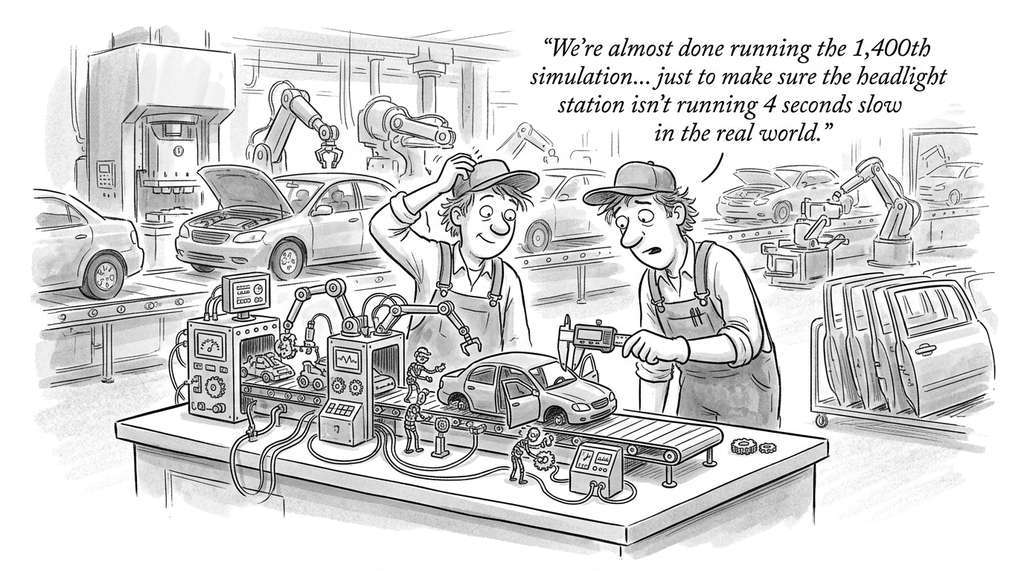
Major automakers, Toyota among them, have reportedly used discrete-event simulation to model assembly lines before reconfiguring physical plants. Each station, conveyor, and worker is represented as a SimPy-style resource with measured processing-time distributions. By simulating thousands of shift schedules and part-arrival sequences, engineers identify bottleneck stations and optimal buffer sizes, saving millions of dollars in trial-and-error rearrangements on the factory floor.
The Segregation Model Nobody Asked For
When Thomas Schelling published his segregation model in 1971, he did not use a computer. He moved pennies and dimes on a checkerboard by hand, flipping coins to decide who moved where. The model he built to explain racial segregation in American cities turned out to explain far more: why similar apps cluster in app stores, why languages form dialect regions, and why even bacteria sort themselves spatially by strain. The mathematics behind it (a Potts model variant, a statistical-physics framework that describes systems of interacting components on a lattice) was not identified until decades later, meaning Schelling accidentally discovered a deep result in condensed-matter physics while studying sociology.
Lab: Queuing Bottleneck Explorer
Goal: Empirically discover how the ratio of service rate to arrival rate (the traffic intensity, denoted \(\rho = \lambda / \mu\), where \(\lambda\) is the arrival rate and \(\mu\) is the service rate) governs queue growth in the screening lab simulation.
Tools needed: Python 3, SimPy, NumPy, Matplotlib (all pip-installable).
Procedure (20 minutes): Using the screening lab code from this section, fix the number of readers at 1 and vary the arrival rate from 0.5/h to 5.0/h in 10 steps. For each arrival rate, run 5 replications (different seeds) for 200 simulated hours and record the mean wait time and p95 wait time.
What to vary: The arrival_rate parameter in the arrivals function.
What to observe: Plot mean wait time vs. arrival rate. You should see wait times remain low until the arrival rate approaches the reader's service rate (~2/h, since reading takes ~0.5h on average), then explode. This is the queuing theory result that wait time diverges as traffic intensity approaches 1.0. Annotate the plot with a vertical line at the theoretical critical arrival rate and compare your empirical curve to the M/M/1 formula (a standard queuing-theory result for a single server with Poisson arrivals and exponential service times): mean wait = 1 / (service_rate - arrival_rate).
7. Summary
Computational experiments turn hypotheses into executable code. Agent-based models capture emergent phenomena by simulating autonomous agents with local rules. Discrete-event simulations capture process dynamics by jumping between events and tracking resource utilization. Both paradigms require careful attention to reproducibility: random seeds, parameter serialization, version control, and statistical replication. Simulators also serve as factories for synthetic data, provided they are properly calibrated. Section 43.2 moves from the macro-scale systems modeled by ABMs and DES to the molecular and chemical scales, where stochastic simulation and molecular dynamics reveal the physics of individual reactions and atomic interactions.
What's Next
Section 43.2: Stochastic Simulation and Molecular Dynamics descends to the molecular scale. The Gillespie algorithm provides exact stochastic simulation of chemical reaction networks, while OpenMM drives molecular dynamics at the atomic level. MDAnalysis then turns raw trajectories into scientifically meaningful observables.