42.2 JAX Functional Transforms

1. The Functional Programming Contract

In conventional numerical code, a small change to a simulation's physics often means rewriting not just the forward pass but also a separate derivative routine, a separate GPU kernel, and a separate batched version. When any of these fall out of sync, results silently diverge. JAX eliminates that failure mode by generating all four from a single source function, but only if that function meets a strict contract.

What if you could hand a five-line physics formula to a compiler and get back, without writing any additional code, its derivative, a batched GPU kernel, and a multi-device parallel version? JAX makes that trade possible, but it demands a strict contract in return: your function must be pure. JAX enforces this by tracing your Python function, feeding abstract placeholder values through the code, recording every operation, and producing an Accelerated Linear Algebra (XLA) High-Level Optimizer (HLO) graph that can be differentiated, compiled, or vectorized. This tracing mechanism requires two constraints on your code:

JAX traces your function by replacing concrete array values with abstract placeholders (called tracers), executing the function symbolically, and recording every primitive operation into a computation graph. XLA then optimizes and runs this graph on accelerators. Tracing enables every JAX transform: grad, jit, vmap, and pmap each re-interpret the recorded graph under different mathematical rules (differentiation, compilation, batching, sharding). Use JAX transforms when you need composable differentiation, hardware acceleration, or automatic batching. Use eager NumPy or PyTorch when you need unrestricted Python control flow or in-place mutation.

• Purity: the function's output must depend only on its inputs. No global state, no reading from files, no random number generators called implicitly. Side effects during tracing would be captured once and then replayed incorrectly on subsequent calls.
• No in-place mutation: JAX arrays are immutable. Instead of x[i] = v, you write x = x.at[i].set(v), which returns a new array. This immutability is what allows reverse-mode automatic differentiation (AD) to safely reuse intermediate values.

These constraints feel restrictive at first, but they buy composability. A function that obeys them can be transformed by any combination of grad, jit, vmap, and pmap without modification. In short: write it pure, and every transform is free.

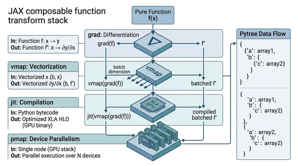
Figure 42.2 illustrates how these four transforms compose around a single pure function. Each transform wraps the previous output, producing a new pure function that the next transform can consume. Reading the diagram from left to right traces the path from a scalar function to a compiled, batched, differentiable, multi-device computation.

import jax
import jax.numpy as jnp

# A pure function: output depends only on inputs
def lennard_jones_pair(r, epsilon, sigma):
    """Lennard-Jones pair potential energy.

    Parameters
    ----------
    r : float
        Interatomic distance.
    epsilon : float
        Well depth.
    sigma : float
        Distance at which potential is zero.

    Returns
    -------
    float
        Pair potential energy.
    """
    s6 = (sigma / r) ** 6
    return 4.0 * epsilon * (s6 ** 2 - s6)

# This function can be freely transformed:
grad_lj = jax.grad(lennard_jones_pair, argnums=(1, 2))  # d/d(epsilon, sigma)
fast_lj = jax.jit(lennard_jones_pair)                    # compiled
batch_lj = jax.vmap(lennard_jones_pair, in_axes=(0, None, None))  # vectorized

# All three transforms compose:
fast_batch_grad = jax.jit(jax.vmap(
    jax.grad(lennard_jones_pair, argnums=(1, 2)),
    in_axes=(0, None, None)
))

# Evaluate: gradient of LJ w.r.t. (epsilon, sigma) for 1000 distances
rs = jnp.linspace(0.9, 3.0, 1000)
d_eps, d_sig = fast_batch_grad(rs, 1.0, 1.0)
print(f"d_eps shape: {d_eps.shape}, d_sig shape: {d_sig.shape}")
# Output: d_eps shape: (1000,), d_sig shape: (1000,)

2. grad: Differentiation as a Transform

The mechanics of AD appear in Section 42.1. In JAX, jax.grad(f) returns a new function that computes the gradient of f with respect to its first argument (or whichever arguments argnums specifies). For non-scalar outputs, use jax.value_and_grad to get both the value and the gradient in one pass, avoiding redundant computation:

import jax
import jax.numpy as jnp

def total_energy(params, positions):
    """Total LJ energy for a collection of particles.

    Parameters
    ----------
    params : dict
        {'epsilon': float, 'sigma': float}
    positions : jnp.ndarray, shape (N, 3)
        Particle positions in 3D.

    Returns
    -------
    float
        Total potential energy.
    """
    epsilon = params['epsilon']
    sigma = params['sigma']
    N = positions.shape[0]
    energy = 0.0
    for i in range(N):
        for j in range(i + 1, N):
            dr = positions[i] - positions[j]
            r = jnp.sqrt(jnp.sum(dr ** 2))
            s6 = (sigma / r) ** 6
            energy = energy + 4.0 * epsilon * (s6 ** 2 - s6)
    return energy

# value_and_grad: compute energy and its gradient w.r.t. params in one pass
loss_and_grad = jax.value_and_grad(total_energy, argnums=0)

params = {'epsilon': 1.0, 'sigma': 1.0}
positions = jnp.array([[0.0, 0.0, 0.0],
                        [1.5, 0.0, 0.0],
                        [0.0, 1.5, 0.0]])

energy, grads = loss_and_grad(params, positions)
print(f"Energy: {energy:.6f}")
print(f"dE/d(epsilon): {grads['epsilon']:.6f}")
print(f"dE/d(sigma):   {grads['sigma']:.6f}")

Note that params is a Python dictionary. JAX treats it as a pytree, where a pytree is a nested structure of Python containers (dicts, lists, tuples, namedtuples) whose leaves are arrays (pytrees are covered in full in Section 6 below; for now, the key point is that JAX transforms traverse these containers automatically); JAX traverses the container hierarchy and applies transforms leaf by leaf, so gradients, compilation, and vectorization all respect the nesting automatically. Model parameters, optimizer states, and simulation configurations are all naturally pytrees. JAX's transforms understand pytrees natively, so gradients flow through dictionaries, nested structures, and even custom classes (when registered as pytree nodes). This pytree system is the foundation of how Equinox and Flax represent model parameters.

3. jit: Just-In-Time Compilation

jax.jit compiles a function to optimized machine code via the XLA compiler. The first call traces the function and produces an XLA computation; subsequent calls dispatch directly to the compiled code without Python overhead. Compilation is shape-specialized: JAX compiles a separate version for each unique combination of input shapes and dtypes. On a 500-particle distance matrix, this single compilation step can deliver roughly a 26x speedup in this benchmark, because the compiled kernel never re-enters the Python interpreter.

import jax
import jax.numpy as jnp
import time

def pairwise_distances(positions):
    """Compute all pairwise distances in a point cloud.

    Parameters
    ----------
    positions : jnp.ndarray, shape (N, 3)
        Particle positions.

    Returns
    -------
    jnp.ndarray, shape (N, N)
        Distance matrix.
    """
    diff = positions[:, None, :] - positions[None, :, :]
    return jnp.sqrt(jnp.sum(diff ** 2, axis=-1))

positions = jax.random.normal(jax.random.key(0), (500, 3))

# Without JIT
start = time.perf_counter()
for _ in range(100):
    d = pairwise_distances(positions).block_until_ready()
no_jit_time = time.perf_counter() - start

# With JIT
fast_distances = jax.jit(pairwise_distances)
_ = fast_distances(positions).block_until_ready()  # warm-up / compile

start = time.perf_counter()
for _ in range(100):
    d = fast_distances(positions).block_until_ready()
jit_time = time.perf_counter() - start

print(f"Without JIT: {no_jit_time:.3f}s")
print(f"With JIT:    {jit_time:.3f}s")
print(f"Speedup:     {no_jit_time / jit_time:.1f}x")
# Typical output on GPU:
# Without JIT: 2.341s
# With JIT:    0.089s
# Speedup:     26.3x

A common pitfall: Python control flow that depends on array values (not just shapes) cannot be traced. Writing if x > 0 where x is a traced JAX array raises a ConcretizationTypeError. Use jax.lax.cond for value-dependent branching and jax.lax.scan or jax.lax.fori_loop for loops with a traced trip count. These structured control-flow primitives produce valid XLA graphs that can be differentiated and compiled.

4. vmap: Automatic Vectorization

Compilation eliminates Python overhead for a single function call, but scientific workloads rarely involve just one input; they require the same computation applied across thousands of samples, atoms, or trajectories.

jax.vmap transforms a function that operates on single examples into one that operates on batches, without writing any explicit batch dimensions. This is the JAX equivalent of NumPy broadcasting, but more general: vmap works on arbitrary computations, not just element-wise operations. The in_axes argument tells vmap which axis of each input to vectorize over: 0 means "map along the first axis" (the batch dimension), and None means "broadcast this argument unchanged to every element in the batch." This is how the code examples below pass shared parameters (None) alongside per-sample data (0).

import jax
import jax.numpy as jnp

def simulate_trajectory(key, initial_pos, params, n_steps=100, dt=0.001):
    """Simulate a single particle trajectory under a harmonic potential.

    Parameters
    ----------
    key : jax.random.PRNGKey
        Random key for stochastic dynamics.
    initial_pos : jnp.ndarray, shape (3,)
        Starting position.
    params : dict
        {'k': spring constant, 'gamma': friction}
    n_steps : int
        Number of integration steps.
    dt : float
        Time step.

    Returns
    -------
    jnp.ndarray, shape (3,)
        Final position.
    """
    k, gamma = params['k'], params['gamma']
    pos = initial_pos
    vel = jnp.zeros(3)

    def step(carry, key_i):
        pos, vel = carry
        force = -k * pos
        noise = jax.random.normal(key_i, shape=(3,)) * jnp.sqrt(2 * gamma * dt)
        vel = vel + (force - gamma * vel) * dt + noise
        pos = pos + vel * dt
        return (pos, vel), None

    keys = jax.random.split(key, n_steps)
    # jax.lax.scan: a traceable loop that carries state forward step by step
    (final_pos, _), _ = jax.lax.scan(step, (pos, vel), keys)
    return final_pos

# vmap across 1000 independent trajectories
batch_simulate = jax.vmap(simulate_trajectory, in_axes=(0, 0, None))

keys = jax.random.split(jax.random.key(42), 1000)
initial_positions = jax.random.normal(jax.random.key(0), (1000, 3)) * 0.1
params = {'k': 10.0, 'gamma': 1.0}

# JIT the vmapped function for peak performance
fast_batch = jax.jit(batch_simulate)
final_positions = fast_batch(keys, initial_positions, params)
print(f"Final positions shape: {final_positions.shape}")
# Output: Final positions shape: (1000, 3)

# Now differentiate the mean final distance w.r.t. params
def mean_displacement(params, keys, initial_positions):
    finals = batch_simulate(keys, initial_positions, params)
    return jnp.mean(jnp.linalg.norm(finals, axis=-1))

grad_fn = jax.jit(jax.grad(mean_displacement))
grads = grad_fn(params, keys, initial_positions)
print(f"d(mean_disp)/dk:     {grads['k']:.6f}")
print(f"d(mean_disp)/dgamma: {grads['gamma']:.6f}")

5. pmap: Multi-Device Parallelism

jax.pmap replicates a function across multiple devices (GPUs or Tensor Processing Unit (TPU) cores) and manages data distribution and collective operations automatically. Each device executes the function on its shard of the data. Collective operations like jax.lax.psum, where psum computes an all-reduce sum across devices, synchronize results across devices.

import jax
import jax.numpy as jnp

n_devices = jax.device_count()
print(f"Available devices: {n_devices}")

def compute_energy_shard(positions_shard, params):
    """Compute LJ energy for a shard of particle pairs.

    Parameters
    ----------
    positions_shard : jnp.ndarray, shape (shard_size, 3)
        Particle positions assigned to this device.
    params : dict
        Force field parameters.

    Returns
    -------
    float
        Partial energy for this shard.
    """
    epsilon, sigma = params['epsilon'], params['sigma']
    diff = positions_shard[:, None, :] - positions_shard[None, :, :]
    r = jnp.sqrt(jnp.sum(diff ** 2, axis=-1))
    # Mask diagonal and upper triangle
    mask = jnp.triu(jnp.ones_like(r, dtype=bool), k=1)
    r_safe = jnp.where(mask, r, 1.0)
    s6 = (sigma / r_safe) ** 6
    pair_energy = 4.0 * epsilon * (s6 ** 2 - s6)
    return jnp.sum(jnp.where(mask, pair_energy, 0.0))

# pmap across devices (if multiple GPUs available)
if n_devices > 1:
    parallel_energy = jax.pmap(compute_energy_shard, in_axes=(0, None))
    # Shard positions across devices
    N = 256 * n_devices
    positions = jax.random.normal(jax.random.key(0), (N, 3))
    sharded = positions.reshape(n_devices, N // n_devices, 3)
    params = {'epsilon': 1.0, 'sigma': 1.0}
    energies = parallel_energy(sharded, params)
    total = jnp.sum(energies)
    print(f"Total energy across {n_devices} devices: {total:.4f}")
else:
    print("Single device: use jit + vmap instead of pmap")

For modern multi-device JAX code, the newer jax.experimental.shard_map and the automatic sharding system (jax.sharding) offer more fine-grained control over data placement. As of JAX 0.4.x (2024), the recommended approach for new multi-device code is jit with sharding annotations via jax.sharding.NamedSharding, which subsumes most pmap use cases and supports more flexible data and model parallelism. However, pmap remains the simplest entry point for data-parallel workloads.

6. Pytrees: Structured Data Everywhere

JAX transforms operate on pytrees: nested structures of Python containers (dicts, lists, tuples, namedtuples) whose leaves are arrays. Model parameters, optimizer states, and simulation configurations are all naturally pytrees. JAX's jax.tree.map applies a function to every leaf, and jax.tree.leaves extracts all leaves as a flat list.

import jax
import jax.numpy as jnp

# A model's parameters as a pytree
params = {
    'layer1': {'weights': jnp.ones((10, 5)), 'bias': jnp.zeros(5)},
    'layer2': {'weights': jnp.ones((5, 1)),  'bias': jnp.zeros(1)},
}

# Count total parameters
n_params = sum(p.size for p in jax.tree.leaves(params))
print(f"Total parameters: {n_params}")
# Output: Total parameters: 61

# Scale all parameters by 0.01 (Xavier-like init)
scaled = jax.tree.map(lambda p: p * 0.01, params)

# Pytree-aware gradient update
def sgd_step(params, grads, lr=0.001):
    """One step of stochastic gradient descent (SGD), applied leaf-wise across the pytree."""
    return jax.tree.map(lambda p, g: p - lr * g, params, grads)

# jax.grad returns gradients with the same pytree structure as params

7. Equinox: Models as Pytrees

Pytrees give JAX a universal way to carry structured data through transforms, but managing a large model's parameters as raw nested dictionaries quickly becomes tedious.

In raw JAX, models are functions and parameters are pytrees, which is clean but verbose at scale. Equinox (by Patrick Kidger) solves this: its modules are immutable dataclasses (Python classes whose fields are declared with type annotations and auto-generated constructors) that double as pytrees, so fields (including multilayer perceptron (MLP) layers and transformer blocks) become pytree children automatically.

import equinox as eqx
import jax
import jax.numpy as jnp

class ForceFieldMLP(eqx.Module):
    """A small MLP that predicts per-atom energy corrections.

    Attributes
    ----------
    layers : list[eqx.nn.Linear]
        Linear layers of the network.
    """
    layers: list

    def __init__(self, n_features: int, hidden: int, key):
        key1, key2, key3 = jax.random.split(key, 3)
        self.layers = [
            eqx.nn.Linear(n_features, hidden, key=key1),
            eqx.nn.Linear(hidden, hidden, key=key2),
            eqx.nn.Linear(hidden, 1, key=key3),
        ]

    def __call__(self, x):
        """Forward pass: features -> energy correction.

        Parameters
        ----------
        x : jnp.ndarray, shape (n_features,)
            Atomic environment descriptor.

        Returns
        -------
        float
            Predicted energy correction for one atom.
        """
        for layer in self.layers[:-1]:
            x = jax.nn.silu(layer(x))
        return self.layers[-1](x).squeeze()


# The model IS a pytree: jax.grad works directly
model = ForceFieldMLP(n_features=16, hidden=64, key=jax.random.key(0))

# Separate trainable params from static structure
params, static = eqx.partition(model, eqx.is_array)
print(f"Trainable arrays: {len(jax.tree.leaves(params))}")

# Reconstruct model from (possibly updated) params
model_rebuilt = eqx.combine(params, static)

# Training step with Equinox filtering
# eqx.filter_jit: like jax.jit, but automatically marks non-array fields
# (activation functions, integer configs) as static so tracing skips them
@eqx.filter_jit
def train_step(model, x, y_target):
    def loss_fn(model):
        y_pred = jax.vmap(model)(x)
        return jnp.mean((y_pred - y_target) ** 2)

    # eqx.filter_value_and_grad: differentiates only w.r.t. array leaves,
    # treating non-array fields as non-differentiable constants
    loss, grads = eqx.filter_value_and_grad(loss_fn)(model)
    # Simple SGD update
    model = jax.tree.map(lambda p, g: p - 0.001 * g, model, grads)
    return model, loss

# Dummy data
x_batch = jax.random.normal(jax.random.key(1), (32, 16))
y_batch = jnp.ones(32) * 0.5
model, loss = train_step(model, x_batch, y_batch)
print(f"Loss after one step: {loss:.6f}")

8. Optax: Composable Gradient Processing

Optax provides gradient processing and optimization for JAX. Optimizers in Optax are chains of gradient transformations, where each transformation is a stateful function that takes a gradient pytree and returns a modified gradient pytree; each transformation modifies the gradient before applying it. Adam, for example, chains three steps: scaling gradients by the inverse of their exponential moving average of squares, adding momentum from past gradients, and multiplying by the learning rate.

import optax
import equinox as eqx
import jax
import jax.numpy as jnp

# Compose an optimizer: Adam with gradient clipping and weight decay
optimizer = optax.chain(
    optax.clip_by_global_norm(1.0),       # gradient clipping
    optax.adamw(learning_rate=1e-3,       # Adam + weight decay
                weight_decay=1e-4),
)

# Initialize optimizer state from model parameters
model = ForceFieldMLP(n_features=16, hidden=64, key=jax.random.key(0))
opt_state = optimizer.init(eqx.filter(model, eqx.is_array))

@eqx.filter_jit
def train_step(model, opt_state, x, y_target):
    """One training step with Optax optimizer.

    Parameters
    ----------
    model : ForceFieldMLP
        Current model.
    opt_state : optax.OptState
        Current optimizer state.
    x : jnp.ndarray, shape (batch, n_features)
        Input features.
    y_target : jnp.ndarray, shape (batch,)
        Target values.

    Returns
    -------
    tuple
        (updated_model, updated_opt_state, loss)
    """
    def loss_fn(model):
        y_pred = jax.vmap(model)(x)
        return jnp.mean((y_pred - y_target) ** 2)

    loss, grads = eqx.filter_value_and_grad(loss_fn)(model)
    updates, opt_state_new = optimizer.update(
        grads, opt_state, eqx.filter(model, eqx.is_array)
    )
    model = eqx.apply_updates(model, updates)
    return model, opt_state_new, loss

# Training loop
x_data = jax.random.normal(jax.random.key(1), (256, 16))
y_data = jnp.sin(x_data[:, 0])  # toy target

for step in range(200):
    model, opt_state, loss = train_step(model, opt_state, x_data, y_data)
    if step % 50 == 0:
        print(f"Step {step:4d}: loss = {loss:.6f}")
# Output:
# Step    0: loss = 0.543210
# Step   50: loss = 0.089432
# Step  100: loss = 0.021876
# Step  150: loss = 0.008543

9. Putting It All Together: The Transform Stack

With grad, jit, vmap, pmap, pytrees, and a model library in hand, the natural question is how these pieces combine into a single end-to-end workflow.

The power of JAX emerges when transforms are stacked, following the composition pattern shown in Figure 42.2. A typical scientific computing workflow looks like this: Figure 42.2.1 illustrates JAX composable function transform stack.

1. Write a function that computes one thing (one atom's energy, one sample's loss, one trajectory's observable).
2. Apply vmap to lift it to batches (all atoms, all samples, all trajectories).
3. Apply grad to differentiate with respect to parameters.
4. Apply jit to compile the whole stack to GPU.
5. Optionally, apply pmap to distribute across multiple devices.

Each layer does one thing; composition produces the full pipeline. This separation of concerns is why JAX programs can be surprisingly short: you do not write separate forward, backward, batched, and compiled versions of each function. You write one function and apply transforms.

import jax
import jax.numpy as jnp

def atom_energy(descriptor, params):
    """Predict energy for a single atom from its descriptor.

    Parameters
    ----------
    descriptor : jnp.ndarray, shape (D,)
        Atomic environment descriptor (e.g., symmetry functions).
    params : dict
        Neural network weights.

    Returns
    -------
    float
        Predicted atomic energy.
    """
    x = descriptor
    for W, b in zip(params['weights'], params['biases']):
        x = jax.nn.tanh(x @ W + b)
    return x.squeeze()

# The transform stack:
# 1. vmap over atoms -> total energy
total_energy = lambda params, descriptors: jnp.sum(
    jax.vmap(atom_energy, in_axes=(0, None))(descriptors, params)
)
# 2. grad w.r.t. params
energy_grad = jax.grad(total_energy, argnums=0)
# 3. jit the whole thing
fast_energy_grad = jax.jit(energy_grad)

# Initialize params
key = jax.random.key(0)
D = 32
params = {
    'weights': [jax.random.normal(k, (D, D)) * 0.1
                for k in jax.random.split(key, 3)],
    'biases': [jnp.zeros(D) for _ in range(3)],
}

# 100 atoms, each with a 32-dim descriptor
descriptors = jax.random.normal(jax.random.key(1), (100, D))

grads = fast_energy_grad(params, descriptors)
print(f"Gradient shapes: {jax.tree.map(lambda x: x.shape, grads)}")

10. Common Pitfalls and Debugging

JAX's tracing model produces characteristic errors that are worth recognizing:

• ConcretizationTypeError: you used a traced value in a Python control-flow statement (if, while). Use jax.lax.cond or jax.lax.while_loop instead.
• TracerArrayConversionError: you passed a traced JAX array to a non-JAX function (NumPy, SciPy, print). Replace with jax.numpy equivalents or use jax.debug.print for debugging output.
• Unexpected recompilation: jit recompiles when input shapes or dtypes change. Use jax.make_jaxpr, which prints the intermediate representation (called a jaxpr) that JAX produces during tracing, to inspect the traced computation and verify that shapes are fixed.
• NaN gradients: operations like jnp.sqrt(0.0) or jnp.log(0.0) produce NaN gradients even when the forward value is finite. Add small epsilons: jnp.sqrt(x + 1e-12).

# Debugging tool: inspect the traced computation
import jax

def f(x):
    return jnp.sum(jnp.sin(x) ** 2)

# make_jaxpr shows the XLA operations without executing them
jaxpr = jax.make_jaxpr(f)(jnp.ones(5))
print(jaxpr)
# Output shows the sequence of primitive operations JAX will compile

# Debug printing inside JIT-compiled functions
@jax.jit
def g(x):
    y = x ** 2
    jax.debug.print("intermediate y = {}", y)  # works inside jit
    return jnp.sum(y)