42.3 Differentiable Physics and Molecular Dynamics

1. The ODE-Constrained Optimization Problem

Without a way to propagate sensitivity through a simulation, every parameter tweak demands a full rerun; for a million-step molecular dynamics trajectory, that means weeks of compute per candidate force field. The adjoint method collapses that cost to a single backward pass, making gradient-based calibration practical for problems that were previously intractable.

Many scientific discovery problems have the following structure. We have a dynamical system governed by an ordinary differential equation (ODE):

where \(z(t) \in \mathbb{R}^d\) is the state (particle positions and velocities, field values, concentrations), \(\theta \in \mathbb{R}^p\) are parameters we want to optimize (force field coefficients, reaction rates, material properties), and \(f\) is the dynamics function. We observe some quantity at the end of the simulation:

and we want \(\nabla_\theta L\): how does the loss change when we adjust the parameters? This is ODE-constrained optimization, and it is the mathematical backbone of differentiable physics.

Formal Definition and When to Use It

ODE-constrained optimization finds parameters \(\theta\) that minimize a loss \(L(\theta)\) when \(L\) depends on \(\theta\) only through a differential equation's solution. It matters because nearly every physical simulation, from climate models to drug binding trajectories, solves differential equations whose parameters we tune to match experimental data. The approach treats the ODE as a constraint and propagates sensitivity information through the dynamics to compute \(\nabla_\theta L\). Two directions are possible: forward (tangent method, cost \(O(p)\) per parameter) or backward (adjoint method, cost independent of parameter count). Use ODE-constrained optimization when the simulation is differentiable and the parameter count \(p\) is moderate to large; for non-differentiable or chaotic simulations, prefer gradient-free approaches such as Bayesian optimization or evolutionary strategies (covered in Chapter 45).

2. Naive Approach: Backpropagation Through Time

If we discretize the ODE with \(N\) time steps using a simple Euler integrator:

then the full computation is a chain of \(N\) differentiable operations. Standard reverse-mode automatic differentiation (AD) (backpropagation) stores all intermediate states \(z_0, z_1, \ldots, z_N\) and walks backward through the chain to compute the gradient. This produces exact gradients but requires \(O(N \cdot d)\) memory for the trajectory. For molecular dynamics with \(N = 10^5\) steps and \(d = 3 \times 10^4\) atoms, this is hundreds of gigabytes, far exceeding GPU memory.

Gradient checkpointing (discussed in Section 42.1) reduces the memory to \(O(\sqrt{N} \cdot d)\) at the cost of recomputation, but the adjoint method offers a more elegant solution that is particularly natural for ODEs.

3. The Continuous Adjoint Method

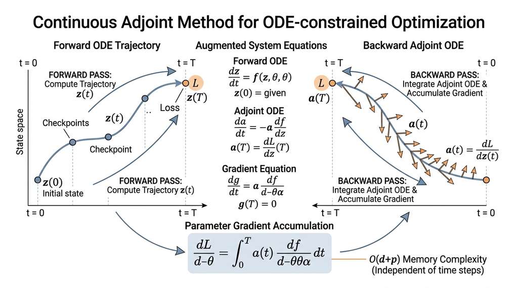
The adjoint method reformulates the gradient computation as a backward ODE that runs in constant memory, regardless of the number of time steps. The derivation proceeds in three steps. Figure 42.3 below illustrates the complete data flow from forward simulation through the backward adjoint pass.

Step 1: Define the adjoint variable. Let \(a(t) = \frac{\partial L}{\partial z(t)} \in \mathbb{R}^d\) be the sensitivity of the loss with respect to the state at time \(t\). At the final time, we know \(a(T) = \frac{\partial \ell}{\partial z(T)}\).

Step 2: Derive the adjoint ODE. By the chain rule, the adjoint evolves backward in time according to:

This is the transpose of the forward dynamics' Jacobian, applied to the adjoint. In the language of Section 42.1, it is a continuous-time vector-Jacobian product (VJP), where the Jacobian \(\partial f / \partial z\) is the matrix of partial derivatives of the dynamics with respect to the state: the adjoint at each instant is the VJP of the adjoint with the dynamics Jacobian.

Step 3: Accumulate parameter gradients. The gradient with respect to \(\theta\) is obtained by integrating along the backward trajectory:

In practice, rather than solving three separate equations, we combine the state \(z\), the adjoint \(a\), and the running parameter gradient \(dL/d\theta\) into a single "augmented" system and integrate it backward in one pass:

starting from \(t = T\) with initial conditions \((z(T), a(T), 0)\) and integrating to \(t = 0\). The state \(z(t)\) can be reconstructed by solving the forward ODE backwards (or by using checkpoints for numerical stability), so the method requires only \(O(d + p)\) memory: the current state, the current adjoint, and the accumulated parameter gradient, as shown in Figure 42.3. For a 30,000-atom system over 100,000 steps, naive backpropagation demands hundreds of gigabytes; the adjoint method typically needs on the order of hundreds of kilobytes. In short: the adjoint method turns "solve the whole simulation again for every parameter" into "solve one backward ODE once for all parameters." Figure 42.3.1 illustrates the continuous adjoint method for ODE-constrained optimization.

Mental Model

Think of the adjoint method like tracing a river upstream to find the source of contamination. A factory downstream (the loss function) detects a chemical at concentration \(C\). You could sample the water at every meter along the entire river, store every sample, and then walk backward through your samples to find where the contaminant entered (backpropagation through time). That works, but you need a warehouse of sample bottles. The adjoint method instead launches a single sensor boat at the factory that reads the current at each point and rides upstream, continuously updating its estimate of where the contamination originates. The boat carries only its current reading and its running tally of candidate sources (the adjoint state and the accumulated parameter gradient), never needing to store the state of the entire river. It arrives at the headwaters with the same answer, having carried only a small notebook instead of a warehouse.

4. Implementing the Adjoint Method with diffrax

The diffrax library (by Patrick Kidger) provides differentiable ODE and stochastic differential equation (SDE) solvers in JAX. It supports multiple adjoint methods out of the box: direct backpropagation through the solver steps, the continuous adjoint, and recursive checkpointing. Here we solve a simple damped oscillator and compute gradients of a trajectory observable with respect to the damping coefficient.

import jax
import jax.numpy as jnp
import diffrax

def damped_oscillator(t, state, args):
    """Dynamics of a damped harmonic oscillator.

    Parameters
    ----------
    t : float
        Current time (unused for autonomous system).
    state : jnp.ndarray, shape (2,)
        [position, velocity].
    args : dict
        {'k': spring constant, 'gamma': damping coefficient}

    Returns
    -------
    jnp.ndarray, shape (2,)
        [velocity, acceleration].
    """
    x, v = state
    k, gamma = args['k'], args['gamma']
    return jnp.array([v, -k * x - gamma * v])

def simulate_and_observe(params):
    """Simulate a damped oscillator and return the final displacement.

    Parameters
    ----------
    params : dict
        {'k': float, 'gamma': float}

    Returns
    -------
    float
        Squared final displacement (the observable we optimize).
    """
    state0 = jnp.array([1.0, 0.0])  # start displaced, at rest

    solver = diffrax.Tsit5()         # Tsitouras 5th-order method
    term = diffrax.ODETerm(damped_oscillator)
    saveat = diffrax.SaveAt(t1=True)

    # Use RecursiveCheckpointAdjoint for memory-efficient gradients
    adjoint = diffrax.RecursiveCheckpointAdjoint()

    sol = diffrax.diffeqsolve(
        term, solver,
        t0=0.0, t1=10.0, dt0=0.01,
        y0=state0, args=params,
        saveat=saveat,
        adjoint=adjoint,
    )
    final_state = sol.ys[-1]
    return final_state[0] ** 2  # squared final displacement

# Gradient of the observable w.r.t. damping and spring constant
grad_fn = jax.jit(jax.grad(simulate_and_observe))

params = {'k': 1.0, 'gamma': 0.5}
grads = grad_fn(params)
print(f"d(x_final^2)/dk:     {grads['k']:.8f}")
print(f"d(x_final^2)/dgamma: {grads['gamma']:.8f}")

# Verify with finite differences
import copy
h = 1e-5
for name in ['k', 'gamma']:
    p_plus = copy.copy(params)
    p_plus[name] = params[name] + h
    p_minus = copy.copy(params)
    p_minus[name] = params[name] - h
    fd = (simulate_and_observe(p_plus) - simulate_and_observe(p_minus)) / (2 * h)
    print(f"d(x_final^2)/d{name} [finite diff]: {fd:.8f}")

The RecursiveCheckpointAdjoint combines the adjoint method with optimal checkpointing: it stores \(O(\log N)\) intermediate states and recomputes the rest, giving both memory efficiency and numerical stability. For long simulations (\(N > 10^4\) steps), this is dramatically cheaper than storing the full trajectory.

5. Differentiable Molecular Dynamics with JAX-MD

The adjoint method and diffrax handle generic ODE plumbing, but a real physical system adds thousands of interacting particles, neighbor lists, and periodic boundary conditions.

JAX-MD (Schoenholz and Cubuk, 2020) is a molecular dynamics library built entirely in JAX. Molecular dynamics is a particularly natural fit for differentiable programming because its core operations (computing pairwise distances, evaluating smooth potential energy functions, deriving forces as gradients of energy) are already differentiable by construction; the simulation is a long chain of these smooth operations, so AD can propagate sensitivity through the entire trajectory without special handling. Because every operation (neighbor list construction, force computation, integration) is a JAX function, the entire MD simulation is automatically differentiable. This means you can compute gradients of any trajectory-averaged observable (energy, pressure, RDF) with respect to force field parameters.

import jax
import jax.numpy as jnp
from jax_md import space, energy, simulate, quantity, partition

# Set up a periodic simulation box
box_size = 10.0
displacement_fn, shift_fn = space.periodic(box_size)

# Define a Lennard-Jones potential with learnable parameters
def lj_energy_fn(dr, epsilon=1.0, sigma=1.0):
    """Lennard-Jones pair energy as a function of distance.

    Parameters
    ----------
    dr : float
        Pairwise distance.
    epsilon : float
        Well depth parameter.
    sigma : float
        Length scale parameter.

    Returns
    -------
    float
        Pair interaction energy.
    """
    idr6 = (sigma / dr) ** 6
    return 4.0 * epsilon * (idr6 ** 2 - idr6)

# Build the neighbor list for efficient pair enumeration
key = jax.random.key(0)
N = 64
positions = jax.random.uniform(key, (N, 3)) * box_size

# JAX-MD energy function from pair potential
energy_fn = energy.pair(
    lj_energy_fn,
    displacement_or_metric=displacement_fn,
    sigma=1.0,
    epsilon=1.0,
)

# Neighbor list for O(N) force computation
neighbor_fn = partition.neighbor_list(
    displacement_fn,
    box=box_size,
    r_cutoff=2.5,
    capacity_multiplier=1.5,
)
neighbors = neighbor_fn.allocate(positions)

# Compute energy and forces
E = energy_fn(positions, neighbor=neighbors)
force_fn = quantity.force(energy_fn)
forces = force_fn(positions, neighbor=neighbors)

print(f"Total energy:  {E:.4f}")
print(f"Forces shape:  {forces.shape}")
print(f"Max force mag: {jnp.max(jnp.linalg.norm(forces, axis=-1)):.4f}")

6. Running a Differentiable MD Simulation

JAX-MD provides integrators (Velocity Verlet, a symplectic integrator that updates positions and velocities in a leapfrog pattern to conserve energy over long trajectories, Nose-Hoover, a deterministic thermostat that maintains constant temperature by coupling the system to an auxiliary dynamic variable, and Langevin) that are themselves JAX functions. We can run a short constant particle number, volume, and temperature (NVT) trajectory, compute an observable, and differentiate through the entire simulation.

import jax
import jax.numpy as jnp
from jax_md import simulate, space, energy, partition

def run_nvt_simulation(params, positions, key, n_steps=500, dt=0.001):
    """Run a short NVT (constant number, volume, temperature) simulation and return the mean kinetic energy.

    Parameters
    ----------
    params : dict
        {'epsilon': float, 'sigma': float}
    positions : jnp.ndarray, shape (N, 3)
        Initial particle positions.
    key : jax.random.PRNGKey
        Random key for thermostat noise.
    n_steps : int
        Number of simulation steps.
    dt : float
        Integration time step.

    Returns
    -------
    float
        Time-averaged kinetic energy per particle.
    """
    box_size = 10.0
    displacement_fn, shift_fn = space.periodic(box_size)

    # Build energy function with current parameters
    energy_fn = energy.pair(
        lambda dr, **kwargs: 4.0 * params['epsilon'] * (
            (params['sigma'] / dr) ** 12 - (params['sigma'] / dr) ** 6
        ),
        displacement_or_metric=displacement_fn,
    )

    neighbor_fn = partition.neighbor_list(
        displacement_fn, box=box_size, r_cutoff=2.5 * params['sigma'],
    )
    neighbors = neighbor_fn.allocate(positions)

    # NVT (Nose-Hoover) integrator at target temperature
    kT = 1.0
    init_fn, step_fn = simulate.nvt_nose_hoover(energy_fn, shift_fn, dt, kT)
    state = init_fn(key, positions, neighbor=neighbors)

    # Use lax.scan for a differentiable loop
    def scan_step(carry, _):
        state, nbrs = carry
        state = step_fn(state, neighbor=nbrs)
        ke = quantity.kinetic_energy(state.velocity)
        return (state, nbrs), ke

    (final_state, _), ke_trajectory = jax.lax.scan(
        scan_step, (state, neighbors), None, length=n_steps
    )

    N = positions.shape[0]
    return jnp.mean(ke_trajectory) / N

# Differentiate the mean kinetic energy w.r.t. force field parameters
grad_ke = jax.grad(run_nvt_simulation)

params = {'epsilon': 1.0, 'sigma': 1.0}
key = jax.random.key(42)
positions = jax.random.uniform(jax.random.key(0), (32, 3)) * 10.0

# This backpropagates through 500 MD steps!
grads = grad_ke(params, positions, key)
print(f"d(KE)/d(epsilon): {grads['epsilon']:.6f}")
print(f"d(KE)/d(sigma):   {grads['sigma']:.6f}")

7. Memory Management: Checkpointing Long Trajectories

The jax.lax.scan in Listing 42.17 stores all intermediate states for backpropagation. For long trajectories, wrap the scan body with jax.checkpoint to trade recomputation for memory:

import jax
import functools

def scan_with_checkpointing(f, init, xs, length, checkpoint_every=50):
    """A scan that checkpoints every K steps for memory efficiency.

    Parameters
    ----------
    f : callable
        Step function (carry, x) -> (carry, y).
    init : pytree
        Initial carry value.
    xs : pytree or None
        Inputs scanned over (None if no per-step input).
    length : int
        Number of scan steps.
    checkpoint_every : int
        Checkpoint interval.

    Returns
    -------
    tuple
        (final_carry, stacked_outputs)
    """
    @jax.checkpoint
    def checkpointed_segment(carry, segment_xs):
        return jax.lax.scan(f, carry, segment_xs)

    n_segments = length // checkpoint_every
    remainder = length % checkpoint_every

    if xs is None:
        segments = None
        segment_length = checkpoint_every
    else:
        # Reshape inputs into segments
        segments = jax.tree.map(
            lambda x: x[:n_segments * checkpoint_every].reshape(
                n_segments, checkpoint_every, *x.shape[1:]
            ), xs
        )
        segment_length = checkpoint_every

    # Process segments with checkpointing
    def outer_step(carry, segment_x):
        return checkpointed_segment(carry, segment_x)

    if segments is not None:
        carry, outputs = jax.lax.scan(outer_step, init, segments)
        # Flatten the segmented outputs
        outputs = jax.tree.map(
            lambda x: x.reshape(-1, *x.shape[2:]), outputs
        )
    else:
        # No per-step inputs: use None placeholders
        carry = init
        all_outputs = []
        for _ in range(n_segments):
            carry, seg_out = checkpointed_segment(
                carry, jnp.zeros(checkpoint_every)  # dummy
            )
            all_outputs.append(seg_out)

    return carry, outputs

# Usage: only O(length / checkpoint_every) states stored
# instead of O(length)

8. Beyond ODEs: Differentiable Discrete Simulations

The checkpointing strategies above assume a simulation built from smooth, continuous update steps, but many scientific models rely on discrete events, stochastic sampling, or lattice updates that have no well-defined Jacobian at every point.

Not all physics simulations are continuous ODEs. Discrete event simulations, Monte Carlo samplers, and lattice models require different differentiation strategies. Two approaches extend differentiable programming to these settings:

• Straight-through estimators: replace non-differentiable operations (argmax, discrete sampling) with differentiable approximations during the backward pass. The Gumbel-Softmax trick, a continuous relaxation that approximates sampling from a categorical distribution by adding Gumbel noise and applying a softmax with a temperature parameter, replaces discrete categorical sampling with a smooth surrogate whose temperature controls the approximation quality.
• Score function estimators (REINFORCE): use the identity \(\nabla_\theta \mathbb{E}_{p_\theta}[f(x)] = \mathbb{E}_{p_\theta}[f(x) \nabla_\theta \log p_\theta(x)]\) to estimate gradients through stochastic discrete processes without differentiating through the sampling operation itself.

For molecular simulations specifically, the reparameterization trick, a technique that separates a random variable into a deterministic function of the parameters and an independent noise source so that gradients can flow through the deterministic part, often applies naturally. Langevin dynamics samples positions according to \(x_{t+1} = x_t + \Delta t \, F(x_t)/\gamma + \sqrt{2\Delta t / \gamma} \, \xi_t\) where \(\xi_t \sim \mathcal{N}(0, I)\). Because the noise \(\xi_t\) is independent of the parameters, we can differentiate through the dynamics while treating \(\xi_t\) as fixed. This is exactly what JAX-MD's Langevin integrator does.

9. TorchMD-Net: Neural Network Potentials in PyTorch

The PyTorch ecosystem supports differentiable MD through TorchMD-Net, which implements equivariant neural network potentials, neural networks whose predictions transform correctly under rotations and translations of the input coordinates, preserving physical symmetries, (SchNet, PaiNN, TensorNet) that predict energies and forces from atomic positions and species (as of 2024, TorchMD-Net has expanded to include ET (Equivariant Transformer) and integrates with MACE and other higher-order equivariant models). Where JAX-MD emphasizes composable pair potentials, TorchMD-Net uses message-passing neural networks on atomic graphs.

# TorchMD-Net: neural network potential in PyTorch
# (Shown for comparison; the chapter recipe uses JAX)
import torch
from torchmdnet.models.model import load_model

# Load a pretrained equivariant potential
model = load_model("torchmdnet_ani2x.pt")

# Predict energy and forces
positions = torch.randn(10, 3, requires_grad=True)  # 10 atoms
species = torch.tensor([6, 6, 6, 1, 1, 1, 1, 8, 7, 1])  # C, H, O, N

energy, forces = model(species, positions)
print(f"Energy: {energy.item():.4f} eV")
print(f"Forces shape: {forces.shape}")

# Gradient of energy w.r.t. model parameters for fine-tuning
loss = (energy - target_energy) ** 2
loss.backward()  # standard PyTorch backprop
# model.parameters() now have .grad attributes

10. When Differentiable Physics Breaks Down

Differentiable simulation is powerful but not universal. Several scenarios challenge or defeat gradient-based optimization through physics:

• Chaotic dynamics: in chaotic systems, the gradient \(\partial z(T) / \partial \theta\) grows exponentially with simulation length, producing exploding gradients that are numerically useless. Techniques like least-squares shadowing, a method that finds a nearby trajectory whose time-averaged gradient is well-defined even in chaotic regimes, and ensemble averaging mitigate this for certain classes of chaotic systems.
• Discontinuities: contact events in rigid body physics, phase transitions, and shock waves create discontinuities in the state trajectory. Gradients do not exist at these points. Smooth approximations (soft contact models, diffuse interfaces) or event-driven differentiation are needed.
• Stiff systems (systems where widely separated time scales force explicit integrators to take impractically small steps): implicit integrators for stiff ODEs involve solving nonlinear systems at each step. Differentiating through the nonlinear solve requires implicit differentiation (via the implicit function theorem), which diffrax handles through ImplicitAdjoint.
• Long time horizons: even in non-chaotic systems, gradients through very long trajectories (\(> 10^6\) steps) can suffer from vanishing gradients or accumulating numerical error. The adjoint method with adaptive step-size control is more robust than naive backpropagation, but monitoring gradient norms during training is essential.

For discovery applications, these limitations motivate hybrid approaches: use differentiable simulation for short-horizon optimization (force field fitting, initial condition search) and gradient-free methods (Chapter 45) for problems where gradients are unreliable.