"Forty years of hand-tuned parameterizations, and then a graph neural network trained on the same data beat us at our own game. The atmosphere, it turns out, was waiting for someone to just listen."
An Operational Forecast Model Facing Early Retirement
Numerical Weather Prediction (NWP) solves the primitive equations of atmospheric dynamics on discrete grids. This approach has improved steadily for six decades, but it demands enormous computational resources: the European Centre for Medium-Range Weather Forecasts (ECMWF) Integrated Forecasting System (IFS) runs on thousands of nodes for hours to produce a single 10-day forecast. In 2023, a series of neural network models demonstrated that comparable forecast skill could be achieved in seconds on a single graphics processing unit (GPU), trained purely on historical reanalysis data. The four leading architectures, their training strategies, the physics constraints that make them work, and rigorous evaluation methods are examined below.
1. The Weather Prediction Problem
What. In September 2023, a neural network running on a single GPU produced a 10-day global weather forecast in under 60 seconds, matching the accuracy of a physics-based system that had consumed several hours on a supercomputer with thousands of processors. The problem both systems solve is the same initial-value problem: given the atmospheric state at time \(t\) (temperature, humidity, wind, pressure on a 3D grid), predict the state at time \(t + \Delta t\). Operational centers have traditionally solved this by numerically integrating the primitive equations:
$$\frac{\partial \mathbf{u}}{\partial t} = -(\mathbf{u} \cdot \nabla)\mathbf{u} - \frac{1}{\rho}\nabla p - 2\boldsymbol{\Omega} \times \mathbf{u} + \mathbf{F}$$where \(\mathbf{u}\) is the wind vector, \(p\) is pressure, \(\rho\) is density, \(\boldsymbol{\Omega}\) is Earth's angular velocity, and \(\mathbf{F}\) represents sub-grid forces (turbulence, convection, radiation) that must be parameterized because they occur below the grid resolution.
Accurate weather forecasts are not merely convenient; they are a matter of survival. When operational models underestimate rainfall intensity or misjudge a hurricane's track at the critical 3-to-5-day lead time, the cost is measured in lives lost and billions in damage. That lead-time window is precisely where AI weather models now show their largest gains over traditional systems.
Why AI changes the game. The parameterization bottleneck is the key. Sub-grid physics accounts for the majority of forecast error in traditional NWP models. These parameterizations are hand-tuned, computationally expensive, and structurally limited. Neural networks, trained on decades of reanalysis data, learn these relationships implicitly from observations rather than from simplified theoretical models.
How. All leading AI weather models share a common setup. They are trained on ERA5 reanalysis data (ECMWF's best estimate of the atmospheric state from 1979 to present, on a 0.25-degree global grid with 37 pressure levels). The models learn to map two consecutive atmospheric states to the state 6 hours later, then roll out autoregressively (that is, each predicted time step feeds as input to the next, chaining single-step predictions into a multi-day forecast) for longer forecasts. The primary training objective is typically a latitude-weighted mean squared error between the predicted atmospheric state and the corresponding ERA5 target, sometimes combined with the physics-informed loss terms described in Section 6 below.
What Is Reanalysis Data?
Reanalysis data is a gridded, globally complete reconstruction of past atmospheric states. A modern weather model produces it by assimilating all available historical observations (weather stations, satellites, radiosondes, buoys). It matters because raw observations are sparse and unevenly distributed: the Southern Ocean has almost no ground stations, while Europe has thousands. Reanalysis fills these gaps by blending observations with a physics-based model through data assimilation, yielding a consistent, gap-free dataset on a regular grid. Use reanalysis when you need spatially complete training data with consistent quality across all regions and time periods. Use raw observations when you need ground-truth validation or when the reanalysis model itself may introduce systematic biases.
When. AI weather models are most valuable for medium-range forecasting (3 to 10 days), ensemble generation (producing hundreds of forecast members for uncertainty quantification), and rapid deployment in resource-constrained environments. In short: Decades of reanalysis data encode enough atmospheric regularity that a neural network can learn to forecast weather without ever being shown the governing equations.
Traditional NWP encodes atmospheric physics explicitly in differential equations and solves them numerically. AI weather models encode the same physics implicitly by learning from 40+ years of reanalysis data. Neither approach is purely one or the other: NWP uses parameterizations that are partly empirical, and the best AI models (NeuralGCM) embed a differentiable dynamical core. The discovery is that the atmosphere's dynamics are regular enough that a neural network can learn them from data, without being told the equations. This connects to the representation learning principles of Chapter 26: the network discovers its own internal representation of atmospheric physics.
Common Misconception
A frequent misunderstanding is that AI weather models "solve the equations faster" or simulate the atmosphere's physics at an accelerated rate. They do not. These models are pure pattern-matchers: they learn a statistical mapping from one atmospheric snapshot to the next, without ever representing or integrating differential equations internally. Their speed comes not from faster physics simulation but from replacing the simulation entirely with a single forward pass through a neural network. This distinction matters because it explains both their strengths (speed, implicit capture of complex interactions) and their limitations (no guaranteed conservation of mass or energy, potential drift on time horizons beyond their training data).
2. GraphCast: Graph Neural Networks for Weather
GraphCast (Lam et al., 2023) treats the atmosphere as a graph. The Earth's surface is discretized into a multi-resolution icosahedral mesh (a sphere-covering triangulation built by repeatedly subdividing the faces of a regular icosahedron), with nodes representing grid cells and edges encoding spatial adjacency. The atmospheric state at each node includes temperature, specific humidity, wind components, and geopotential on 37 pressure levels, plus surface variables (mean sea level pressure, 2-meter temperature, 10-meter wind).
The architecture has three stages. An encoder maps the input atmospheric state onto mesh nodes using learned embeddings. A processor runs 16 rounds of message passing on the mesh graph, allowing information to propagate globally. A decoder maps the processed mesh back to the latitude-longitude grid to produce the forecast.
Mental Model
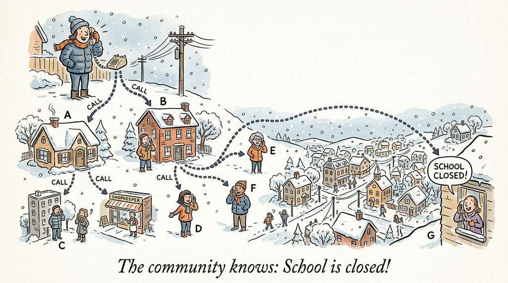
Think of message passing on the mesh graph like a telephone tree during a school snow day. Each parent calls two or three neighbors, who each call their neighbors, and within a few rounds the entire community knows the school is closed. In GraphCast, each mesh node "calls" its neighbors with information about local temperature, wind, and pressure. After 16 rounds of these calls, a node in the western Pacific can incorporate information from the jet stream over North America, because the messages have relayed through intermediate nodes spanning the globe. The multi-resolution mesh acts like having both local neighborhood contacts and long-distance relatives: coarse mesh edges carry information across continents in fewer hops, while fine mesh edges preserve local detail. This is how the model captures teleconnections (distant weather systems influencing each other) without needing to process the entire globe in a single, expensive attention operation.
Figure 51.1 implements the three core components of the GraphCast architecture: the icosahedral mesh construction, the grid-to-mesh encoder, and the message-passing processor.
"""
GraphCast-style mesh graph construction for weather prediction.
We build a multi-resolution icosahedral mesh and map ERA5 grid
points to mesh nodes for message-passing.
"""
import numpy as np
import torch
import torch.nn as nn
from torch_geometric.data import Data


def icosahedral_mesh(refinements: int = 6) -> tuple[np.ndarray, np.ndarray]:
    """Build an icosahedral mesh on the unit sphere.

    Each refinement quadruples the number of faces,
    giving approximately 4^refinements * 20 triangles.

    Returns:
        nodes: (N, 3) array of node positions on the unit sphere
        edges: (2, E) array of edge indices
    """
    # Golden ratio for icosahedron vertices
    phi = (1 + np.sqrt(5)) / 2
    verts = np.array([
        [-1, phi, 0], [1, phi, 0], [-1, -phi, 0], [1, -phi, 0],
        [0, -1, phi], [0, 1, phi], [0, -1, -phi], [0, 1, -phi],
        [phi, 0, -1], [phi, 0, 1], [-phi, 0, -1], [-phi, 0, 1],
    ], dtype=np.float64)
    verts /= np.linalg.norm(verts, axis=1, keepdims=True)

    # 20 triangular faces of the icosahedron
    faces = [
        (0, 11, 5), (0, 5, 1), (0, 1, 7), (0, 7, 10), (0, 10, 11),
        (1, 5, 9), (5, 11, 4), (11, 10, 2), (10, 7, 6), (7, 1, 8),
        (3, 9, 4), (3, 4, 2), (3, 2, 6), (3, 6, 8), (3, 8, 9),
        (4, 9, 5), (2, 4, 11), (6, 2, 10), (8, 6, 7), (9, 8, 1),
    ]

    for _ in range(refinements):
        midpoint_cache = {}
        new_faces = []
        for v0, v1, v2 in faces:
            a = _get_midpoint(v0, v1, verts, midpoint_cache)
            b = _get_midpoint(v1, v2, verts, midpoint_cache)
            c = _get_midpoint(v2, v0, verts, midpoint_cache)
            new_faces.extend([
                (v0, a, c), (v1, b, a), (v2, c, b), (a, b, c)
            ])
            verts = np.array(list(verts) + list(midpoint_cache.values()))
        faces = new_faces

    # Extract unique edges from faces
    edge_set = set()
    for v0, v1, v2 in faces:
        for e in [(v0, v1), (v1, v2), (v2, v0)]:
            edge_set.add((min(e), max(e)))
    edges = np.array(list(edge_set)).T

    return verts[:len(set(i for f in faces for i in f))], edges


def _get_midpoint(v0, v1, verts, cache):
    """Get or create the midpoint between two vertices, projected to sphere."""
    key = (min(v0, v1), max(v0, v1))
    if key not in cache:
        mid = (verts[v0] + verts[v1]) / 2
        mid /= np.linalg.norm(mid)
        cache[key] = mid
    return len(verts) + list(cache.keys()).index(key)


class GraphCastEncoder(nn.Module):
    """Encode ERA5 grid data onto mesh nodes."""

    def __init__(self, grid_features: int, mesh_features: int,
                 hidden_dim: int = 512):
        super().__init__()
        # Grid-to-mesh edges learned during training
        self.grid_mlp = nn.Sequential(
            nn.Linear(grid_features, hidden_dim),
            nn.LayerNorm(hidden_dim),
            nn.SiLU(),
            nn.Linear(hidden_dim, mesh_features),
        )

    def forward(self, grid_data: torch.Tensor) -> torch.Tensor:
        """Map grid features to mesh node embeddings.

        Args:
            grid_data: (batch, n_grid, grid_features)
        Returns:
            mesh_embeddings: (batch, n_grid, mesh_features)
        """
        return self.grid_mlp(grid_data)


class MeshProcessor(nn.Module):
    """Message-passing processor on the icosahedral mesh."""

    def __init__(self, node_dim: int, edge_dim: int, n_layers: int = 16):
        super().__init__()
        self.layers = nn.ModuleList([
            MessagePassingLayer(node_dim, edge_dim)
            for _ in range(n_layers)
        ])

    def forward(self, node_features: torch.Tensor,
                edge_index: torch.Tensor,
                edge_features: torch.Tensor) -> torch.Tensor:
        for layer in self.layers:
            node_features = node_features + layer(
                node_features, edge_index, edge_features
            )
        return node_features


class MessagePassingLayer(nn.Module):
    """Single round of message passing with edge updates."""

    def __init__(self, node_dim: int, edge_dim: int):
        super().__init__()
        self.edge_mlp = nn.Sequential(
            nn.Linear(2 * node_dim + edge_dim, node_dim),
            nn.LayerNorm(node_dim),
            nn.SiLU(),
            nn.Linear(node_dim, edge_dim),
        )
        self.node_mlp = nn.Sequential(
            nn.Linear(node_dim + edge_dim, node_dim),
            nn.LayerNorm(node_dim),
            nn.SiLU(),
            nn.Linear(node_dim, node_dim),
        )

    def forward(self, nodes, edge_index, edges):
        src, dst = edge_index
        # Update edges
        edge_input = torch.cat([nodes[src], nodes[dst], edges], dim=-1)
        edges = edges + self.edge_mlp(edge_input)
        # Aggregate messages and update nodes
        agg = torch.zeros_like(nodes)
        agg.scatter_add_(0, dst.unsqueeze(-1).expand_as(edges), edges)
        node_input = torch.cat([nodes, agg], dim=-1)
        nodes = nodes + self.node_mlp(node_input)
return nodes3. Pangu-Weather: 3D Vision Transformers
While GraphCast uses an explicit mesh, Pangu-Weather (Bi et al., 2023) treats the atmosphere as a 3D volume and processes it with a modified vision Transformer. The key insight is Earth-specific positional encoding: the model learns separate positional embeddings for latitude, longitude, and pressure level, reflecting the fact that atmospheric dynamics have fundamentally different structure in horizontal vs. vertical directions.
Pangu-Weather trains four separate models for 1-hour, 3-hour, 6-hour, and 24-hour lead times. To produce a 7-day forecast, the system chains the 24-hour model seven times rather than rolling out a single 6-hour model 28 times. This reduces error accumulation at the cost of training four models. Figure 51.2 shows how the Earth-specific position encoding decomposes 3D atmospheric coordinates into separate learnable embeddings.
"""
Pangu-Weather-style Earth-specific 3D Transformer block.
The key innovation: separate positional encodings for
horizontal (lat/lon) and vertical (pressure level) axes.
"""
import torch
import torch.nn as nn
import torch.nn.functional as F


class EarthSpecificPositionEncoding(nn.Module):
    """Learnable 3D position encoding decomposed by axis.

    Atmospheric dynamics differ fundamentally between
    horizontal advection and vertical stratification.
    Decomposing the encoding lets the model learn each
    independently.
    """

    def __init__(self, d_model: int, n_lat: int = 721,
                 n_lon: int = 1440, n_levels: int = 13):
        super().__init__()
        self.lat_embed = nn.Embedding(n_lat, d_model // 3)
        self.lon_embed = nn.Embedding(n_lon, d_model // 3)
        self.level_embed = nn.Embedding(n_levels, d_model - 2 * (d_model // 3))
        self.n_lat = n_lat
        self.n_lon = n_lon
        self.n_levels = n_levels

    def forward(self, x: torch.Tensor) -> torch.Tensor:
        """Add position encoding to input tensor.

        Args:
            x: (batch, n_levels, n_lat, n_lon, d_model)
        Returns:
            x with position encoding added
        """
        lat_ids = torch.arange(self.n_lat, device=x.device)
        lon_ids = torch.arange(self.n_lon, device=x.device)
        lev_ids = torch.arange(self.n_levels, device=x.device)

        lat_enc = self.lat_embed(lat_ids)      # (n_lat, d//3)
        lon_enc = self.lon_embed(lon_ids)       # (n_lon, d//3)
        lev_enc = self.level_embed(lev_ids)     # (n_levels, d_rem)

        # Broadcast and concatenate
        pos = torch.cat([
            lat_enc[None, :, None, :].expand(
                self.n_levels, -1, self.n_lon, -1),
            lon_enc[None, None, :, :].expand(
                self.n_levels, self.n_lat, -1, -1),
            lev_enc[:, None, None, :].expand(
                -1, self.n_lat, self.n_lon, -1),
        ], dim=-1)  # (n_levels, n_lat, n_lon, d_model)

        return x + pos.unsqueeze(0)


class PanguBlock(nn.Module):
    """3D Earth-specific Transformer block with window attention.

    Uses shifted window attention (Swin-style, where attention is computed within local windows that shift between layers to enable cross-window connections) adapted for
    the spherical geometry: windows wrap around at the dateline
    and handle polar convergence.
    """

    def __init__(self, d_model: int = 192, n_heads: int = 6,
                 window_size: tuple = (2, 6, 12)):
        super().__init__()
        self.norm1 = nn.LayerNorm(d_model)
        self.attn = nn.MultiheadAttention(d_model, n_heads, batch_first=True)
        self.norm2 = nn.LayerNorm(d_model)
        self.mlp = nn.Sequential(
            nn.Linear(d_model, 4 * d_model),
            nn.GELU(),
            nn.Linear(4 * d_model, d_model),
        )
        self.window_size = window_size

    def forward(self, x: torch.Tensor) -> torch.Tensor:
        """Process atmospheric volume with windowed attention.

        Args:
            x: (batch, n_tokens, d_model) flattened 3D volume
        Returns:
            Updated representations
        """
        # Self-attention with residual
        normed = self.norm1(x)
        attn_out, _ = self.attn(normed, normed, normed)
        x = x + attn_out
        # MLP with residual
        x = x + self.mlp(self.norm2(x))
return xGraphCast and Pangu-Weather both operate in the spatial domain, processing atmospheric variables on grids or meshes; FourCastNet instead asks whether the frequency domain offers a more natural representation of the planetary wave patterns that govern weather.
4. FourCastNet: Adaptive Fourier Neural Operators
FourCastNet (Pathak et al., 2022) takes a spectral approach, building on the Fourier Neural Operator (FNO) architecture covered in Chapter 33. FourCastNet v2 (2023) later replaced the AFNO backbone with a spherical harmonics transformer for improved accuracy at longer lead times. The key modification is the Adaptive Fourier Neural Operator (AFNO), which applies self-attention in the Fourier domain. Standard attention costs \(O(N^2)\) for \(N\) grid points. AFNO instead transforms each channel to the frequency domain, applies a learnable filter, and transforms back. (On a 0.25-degree global grid with roughly one million points, this cuts the mixing cost from a trillion operations to about twenty million: a 50,000-fold reduction.)
This spectral bias is physically motivated. Atmospheric dynamics are dominated by large-scale wave patterns (Rossby waves, where large planetary waves propagate westward due to Earth's rotation, and Kelvin waves) that have clean representations in Fourier space. By operating in the frequency domain, AFNO naturally captures these planetary-scale structures.
Mental Model
Think of AFNO like tuning a graphic equalizer on a stereo system. When you listen to a song in normal playback (spatial domain), adjusting one moment in time affects only that moment. But when you switch to the equalizer view (frequency domain), you see the music decomposed into bass, midrange, and treble bands, and turning a single knob boosts or cuts that frequency everywhere in the song at once. AFNO does the same thing with weather data: it transforms the global atmosphere into its constituent wave patterns (planetary waves in the "bass," storm-scale features in the "treble"), applies learnable filters to amplify or suppress each frequency band, then transforms back. This is why it captures continent-spanning Rossby waves so efficiently: in the frequency domain, a pattern that spans the entire globe is just one coefficient to adjust, not millions of grid points to process individually. The sparsity threshold acts like a noise gate on the equalizer, silencing frequency bands below a certain energy level to keep the forecast clean.
Figure 51.3 implements the AFNO block, showing the 2D FFT, learnable complex-valued MLP, sparsity thresholding, and inverse FFT stages.
"""
Adaptive Fourier Neural Operator (AFNO) block
as used in FourCastNet for weather prediction.
"""
import torch
import torch.nn as nn
import torch.fft


class AFNOBlock(nn.Module):
    """Adaptive Fourier Neural Operator block.

    Performs token mixing in the Fourier domain:
    1. FFT each channel over the spatial dimensions
    2. Apply a learnable complex-valued MLP in frequency space
    3. Inverse FFT back to spatial domain

    This is O(N log N) vs O(N^2) for standard attention,
    and naturally captures the planetary wave structures
    that dominate atmospheric dynamics.
    """

    def __init__(self, d_model: int = 768, n_blocks: int = 8,
                 sparsity_threshold: float = 0.01,
                 hard_threshold: bool = True):
        super().__init__()
        self.d_model = d_model
        self.n_blocks = n_blocks
        self.hard_threshold = hard_threshold
        self.sparsity_threshold = sparsity_threshold

        # Learnable spectral weights (complex-valued)
        self.scale = 0.02
        block_size = d_model // n_blocks
        self.w1 = nn.Parameter(
            self.scale * torch.randn(2, n_blocks, block_size, block_size)
        )
        self.b1 = nn.Parameter(
            self.scale * torch.randn(2, n_blocks, block_size)
        )
        self.w2 = nn.Parameter(
            self.scale * torch.randn(2, n_blocks, block_size, block_size)
        )
        self.b2 = nn.Parameter(
            self.scale * torch.randn(2, n_blocks, block_size)
        )

    def _complex_mul(self, x_real, x_imag, w_real, w_imag):
        """Complex matrix multiplication: (a+bi)(c+di) = (ac-bd) + (ad+bc)i"""
        return (
            torch.einsum("...i,io->...o", x_real, w_real)
            - torch.einsum("...i,io->...o", x_imag, w_imag),
            torch.einsum("...i,io->...o", x_real, w_imag)
            + torch.einsum("...i,io->...o", x_imag, w_real),
        )

    def forward(self, x: torch.Tensor) -> torch.Tensor:
        """Apply AFNO mixing.

        Args:
            x: (batch, height, width, d_model) spatial features
        Returns:
            Mixed features of same shape
        """
        B, H, W, C = x.shape
        block_size = C // self.n_blocks

        # 2D FFT over spatial dimensions
        x_ft = torch.fft.rfft2(x, dim=(1, 2), norm="ortho")

        # Reshape for block-diagonal processing
        x_ft = x_ft.reshape(B, x_ft.shape[1], x_ft.shape[2],
                            self.n_blocks, block_size)

        # Two-layer complex MLP in frequency space
        x_real, x_imag = x_ft.real, x_ft.imag
        for w, b in [(self.w1, self.b1), (self.w2, self.b2)]:
            x_real, x_imag = self._complex_mul(
                x_real, x_imag, w[0], w[1]
            )
            x_real = x_real + b[0]
            x_imag = x_imag + b[1]
            x_real = F.relu(x_real)
            x_imag = F.relu(x_imag)

        # Sparsity: zero out small-magnitude modes
        if self.hard_threshold:
            magnitude = torch.sqrt(x_real ** 2 + x_imag ** 2)
            mask = magnitude > self.sparsity_threshold
            x_real = x_real * mask
            x_imag = x_imag * mask

        # Reconstruct complex tensor and inverse FFT
        x_ft = torch.complex(x_real, x_imag)
        x_ft = x_ft.reshape(B, x_ft.shape[1], x_ft.shape[2], C)
        x = torch.fft.irfft2(x_ft, s=(H, W), dim=(1, 2), norm="ortho")

return x5. NeuralGCM: Hybrid Learned-Physics Models
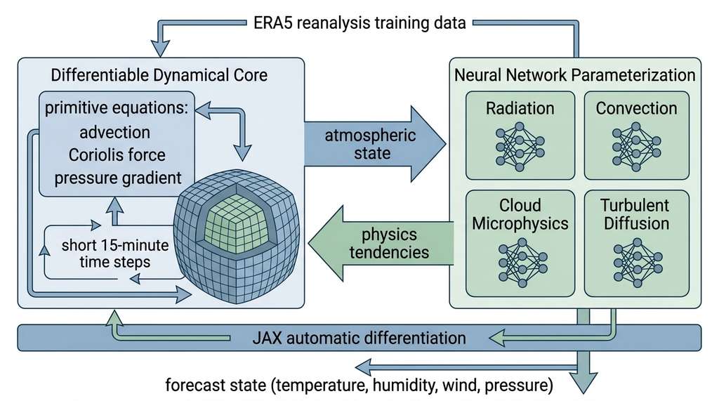
NeuralGCM (Kochkov et al., 2024) diverges from the pure data-driven models. It retains a differentiable dynamical core for the primitive equations and replaces only the sub-grid physics with learned neural networks, preserving conservation laws by construction while letting data teach the hard parts.
The architecture couples a spectral dynamical core (solving the primitive equations on a cubed-sphere grid, where six square patches are mapped onto a sphere to avoid polar singularities) with neural network parameterizations for radiation, convection, cloud microphysics, and turbulent diffusion. The entire system is end-to-end differentiable, trained by backpropagating through both the dynamical core and the neural parameterizations using JAX's automatic differentiation. Figure 51.4 implements a simplified version of this hybrid architecture, with the differentiable dynamical core and learned physics parameterization as separate, composable modules. Figure 51.1.1 illustrates NeuralGCM hybrid architecture.
"""
NeuralGCM-style hybrid model: a differentiable dynamical core
coupled with learned physics parameterizations, implemented in JAX.
"""
import jax
import jax.numpy as jnp
import flax.linen as nn
from typing import NamedTuple


class AtmosphericState(NamedTuple):
    """State vector for the atmospheric model."""
    temperature: jnp.ndarray     # (n_levels, n_lat, n_lon)
    specific_humidity: jnp.ndarray
    u_wind: jnp.ndarray          # zonal wind
    v_wind: jnp.ndarray          # meridional wind
    surface_pressure: jnp.ndarray  # (n_lat, n_lon)


class LearnedPhysics(nn.Module):
    """Neural network parameterization for sub-grid physics.

    Replaces hand-tuned parameterizations for convection,
    radiation, boundary layer turbulence, and cloud microphysics
    with a learned mapping from the resolved state to tendencies.
    """
    hidden_dim: int = 256
    n_levels: int = 37

    @nn.compact
    def __call__(self, column_state: jnp.ndarray) -> jnp.ndarray:
        """Predict physics tendencies for a single atmospheric column.

        Args:
            column_state: (n_levels * n_vars,) concatenated
                temperature, humidity, wind profiles
        Returns:
            tendencies: (n_levels * n_vars,) time derivatives
                from sub-grid processes
        """
        x = nn.Dense(self.hidden_dim)(column_state)
        x = nn.LayerNorm()(x)
        x = nn.silu(x)

        # Two residual blocks
        for _ in range(2):
            residual = x
            x = nn.Dense(self.hidden_dim)(x)
            x = nn.LayerNorm()(x)
            x = nn.silu(x)
            x = nn.Dense(self.hidden_dim)(x)
            x = x + residual

        tendencies = nn.Dense(self.n_levels * 4)(x)  # T, q, u, v
        return tendencies


def spectral_dynamical_core(state: AtmosphericState,
                            dt: float,
                            coriolis: jnp.ndarray) -> AtmosphericState:
    """Differentiable dynamical core solving the primitive equations.

    Simplified version: advection + Coriolis force + pressure gradient.
    The full NeuralGCM uses a spectral transform method on a
    cubed-sphere grid.

    Args:
        state: Current atmospheric state
        dt: Time step in seconds
        coriolis: Coriolis parameter f = 2 * Omega * sin(lat)
    Returns:
        Updated state after one dynamics step
    """
    u, v = state.u_wind, state.v_wind
    T = state.temperature

    # Coriolis acceleration (simplified, on pressure levels)
    du_coriolis = coriolis[None, :, None] * v
    dv_coriolis = -coriolis[None, :, None] * u

    # Horizontal advection (centered differences, periodic in longitude)
    dT_advection = -(
        u * jnp.roll(T, -1, axis=2) - u * jnp.roll(T, 1, axis=2)
    ) / 2.0

    # Update state
    return AtmosphericState(
        temperature=T + dt * dT_advection,
        specific_humidity=state.specific_humidity,
        u_wind=u + dt * du_coriolis,
        v_wind=v + dt * dv_coriolis,
        surface_pressure=state.surface_pressure,
    )


def neuralgcm_step(state: AtmosphericState,
                   physics_model: LearnedPhysics,
                   physics_params: dict,
                   dt_dynamics: float = 900.0,
                   dt_physics: float = 3600.0,
                   coriolis: jnp.ndarray = None) -> AtmosphericState:
    """One time step of the NeuralGCM hybrid model.

    The dynamical core runs at a short time step (15 min),
    and the learned physics is called once per physics time step
    (1 hour), matching the operational practice of traditional GCMs.

    Args:
        state: Current atmospheric state
        physics_model: Learned sub-grid physics parameterization
        physics_params: Flax parameters for the physics model
        dt_dynamics: Dynamics time step (seconds)
        dt_physics: Physics time step (seconds)
        coriolis: Coriolis parameter array
    Returns:
        Updated atmospheric state
    """
    n_substeps = int(dt_physics / dt_dynamics)

    # Multiple dynamics substeps
    for _ in range(n_substeps):
        state = spectral_dynamical_core(state, dt_dynamics, coriolis)

    # Apply learned physics (column-wise)
    n_levels, n_lat, n_lon = state.temperature.shape
    column_inputs = jnp.concatenate([
        state.temperature.reshape(n_levels, -1),
        state.specific_humidity.reshape(n_levels, -1),
        state.u_wind.reshape(n_levels, -1),
        state.v_wind.reshape(n_levels, -1),
    ], axis=0).T  # (n_columns, n_levels * 4)

    tendencies = physics_model.apply(
        physics_params, column_inputs
    )  # (n_columns, n_levels * 4)

    # Unpack and apply tendencies
    t_tend = tendencies[:, :n_levels].T.reshape(n_levels, n_lat, n_lon)
    q_tend = tendencies[:, n_levels:2*n_levels].T.reshape(
        n_levels, n_lat, n_lon)

    return AtmosphericState(
        temperature=state.temperature + dt_physics * t_tend,
        specific_humidity=state.specific_humidity + dt_physics * q_tend,
        u_wind=state.u_wind,
        v_wind=state.v_wind,
        surface_pressure=state.surface_pressure,
)In the 2023 Western Pacific typhoon season, According to evaluations reported by their developers, GraphCast and Pangu-Weather consistently matched or exceeded ECMWF's track forecasts for tropical cyclones at 3 to 7 day lead times. The AI models were particularly strong at predicting recurvature events, where a typhoon's path curves from westward to northeastward. Traditional NWP struggles with recurvature because it depends sensitively on the position of the subtropical ridge, a feature that requires accurate representation of planetary-scale wave patterns. Graph neural networks and vision Transformers, which process the entire global state simultaneously, capture these teleconnections naturally.
NeuralGCM's hybrid design highlights a central tension in all neural weather models: without explicit physical guardrails, a network trained purely on forecast error can silently violate conservation laws and produce internally inconsistent atmospheric states.
6. Physics Constraints in Neural Weather Models
A neural network trained purely to minimize forecast error can violate fundamental physics. It might create or destroy mass, generate energy from nothing, or produce wind fields that are inconsistent with pressure gradients. Three categories of constraints prevent these failures.
6.1 Conservation Laws
The atmosphere conserves total mass, total energy, and (approximately) total moisture. We can enforce these as hard constraints by projecting the network's output onto the constraint manifold (the set of all atmospheric states that satisfy the conservation equations exactly), or as soft constraints by adding penalty terms to the loss function:
where \(M_0\) and \(E_0\) are the initial total mass and energy, \(\rho\) is air density, and \(e\) is specific total energy. Hard constraints are more physically rigorous; soft constraints are easier to implement and more compatible with gradient-based training.
Checkpoint
So far: neural weather models can violate conservation of mass and energy, and we can counter this with hard projection constraints or soft penalty terms in the training loss; next we examine how the energy spectrum and vertical pressure consistency provide two additional physical guardrails.
6.2 Spectral Energy Cascade
Atmospheric kinetic energy flows from large scales to small scales through a turbulent cascade. The kinetic energy spectrum follows an approximate \(k^{-3}\) power law in the synoptic scales (wavelengths of 1000 to 10000 km) and \(k^{-5/3}\) at mesoscales. Neural weather models can develop unrealistic spectral slopes, producing either too-smooth forecasts (insufficient small-scale variability) or spectral artifacts (spurious energy at grid scale). A spectral loss term penalizes deviations from the observed energy spectrum:
$$\mathcal{L}_\text{spectral} = \sum_k \left| \log E(k) - \log E_\text{ERA5}(k) \right|^2$$"""
Spectral energy analysis for verifying that neural weather
models maintain realistic kinetic energy cascades.
"""
import numpy as np
import xarray as xr
from scipy import fft as sp_fft
def kinetic_energy_spectrum(
u: np.ndarray,
v: np.ndarray,
lat: np.ndarray,
) -> tuple[np.ndarray, np.ndarray]:
"""Compute the zonal kinetic energy spectrum.
The atmosphere's kinetic energy follows k^{-3} at synoptic
scales and k^{-5/3} at mesoscales. Neural weather models
that deviate from this spectrum produce unrealistic forecasts.
Args:
u: Zonal wind (lat, lon), m/s
v: Meridional wind (lat, lon), m/s
lat: Latitude array in degrees
Returns:
wavenumbers: Array of zonal wavenumber k
spectrum: Kinetic energy as function of wavenumber, m^2/s^2
"""
n_lon = u.shape[1]
cos_lat = np.cos(np.deg2rad(lat))
# Area-weighted FFT of wind components
u_weighted = u * cos_lat[:, None]
v_weighted = v * cos_lat[:, None]
u_hat = sp_fft.rfft(u_weighted, axis=1)
v_hat = sp_fft.rfft(v_weighted, axis=1)
# Kinetic energy per wavenumber (average over latitudes)
ke_spectrum = np.mean(
np.abs(u_hat) ** 2 + np.abs(v_hat) ** 2, axis=0
) / n_lon ** 2
wavenumbers = np.arange(ke_spectrum.shape[0])
return wavenumbers[1:], ke_spectrum[1:] # skip wavenumber 0
def spectral_loss(
pred_u: np.ndarray,
pred_v: np.ndarray,
target_u: np.ndarray,
target_v: np.ndarray,
lat: np.ndarray,
) -> float:
"""Compute spectral energy loss between predicted and target winds.
Penalizes deviations from the observed kinetic energy spectrum,
preventing the model from producing unrealistically smooth or
noisy forecasts.
Args:
pred_u, pred_v: Predicted wind components
target_u, target_v: ERA5 target wind components
lat: Latitude array
Returns:
Log-spectral energy distance
"""
k, spec_pred = kinetic_energy_spectrum(pred_u, pred_v, lat)
_, spec_target = kinetic_energy_spectrum(target_u, target_v, lat)
# Log-spectral distance, avoiding log(0)
eps = 1e-30
log_ratio = np.log(spec_pred + eps) - np.log(spec_target + eps)
return float(np.mean(log_ratio ** 2))6.3 Pressure-Level Consistency
Atmospheric variables on pressure levels must satisfy hydrostatic balance: the vertical pressure gradient balances gravity. Temperature and geopotential height are linked by the hypsometric equation \(\Delta Z = -\frac{R_d \bar{T}}{g} \ln(p_\text{top}/p_\text{bot})\), where \(R_d\) is the gas constant for dry air, \(\bar{T}\) is the mean layer temperature, and \(g\) is gravitational acceleration. Neural models that predict temperature and geopotential independently can produce physically inconsistent profiles.
Running pretrained AI weather models does not require implementing the architectures above. Google DeepMind's graphcast package provides a JAX implementation with pretrained weights that produce 10-day global forecasts in under a minute on a single TPU. NVIDIA's earth2mip package wraps FourCastNet, Pangu-Weather, and other models behind a unified inference API (as of 2024, NVIDIA's broader Earth-2 platform subsumes earth2mip and adds higher-resolution regional models including CorrDiff for generative downscaling). ECMWF's ai-models package integrates these models into operational workflows. For evaluation, weatherbench2 provides standardized metrics and ERA5 verification data. What took hundreds of lines above reduces to a few configuration calls with these production tools.
7. Evaluation with WeatherBench2
WeatherBench2 (Rasp et al., 2024) is the standard evaluation framework for AI weather models. It provides metrics that match those used by operational centers, ERA5 verification data, and baselines including climatology (the historical average for each day of year) and persistence (tomorrow's weather equals today's). The primary metric is the latitude-weighted root mean square error (RMSE):
$$\text{RMSE}_w = \sqrt{\frac{\sum_i w_i (f_i - o_i)^2}{\sum_i w_i}}$$where \(w_i = \cos(\phi_i)\) weights by the cosine of latitude to account for the convergence of meridians toward the poles, \(f_i\) is the forecast, and \(o_i\) is the ERA5 verification. Additional metrics include the anomaly correlation coefficient (ACC), which measures how well the forecast captures deviations from climatology, and spread-skill ratio (the ratio of ensemble spread to forecast error, where a value of 1.0 indicates a well-calibrated ensemble) for ensemble forecasts.
"""
WeatherBench2-style evaluation metrics for AI weather models.
"""
import numpy as np
import xarray as xr


def latitude_weights(lat: np.ndarray) -> np.ndarray:
    """Compute area-based latitude weights.

    Grid cells near the equator represent more surface area
    than cells near the poles. Cosine-of-latitude weighting
    ensures that global metrics are not biased toward polar
    regions where grid cells are smaller.

    Args:
        lat: Latitude values in degrees
    Returns:
        Normalized weights summing to 1
    """
    weights = np.cos(np.deg2rad(lat))
    return weights / weights.sum()


def weighted_rmse(forecast: xr.DataArray,
                  observation: xr.DataArray,
                  dim: str = "time") -> xr.DataArray:
    """Latitude-weighted RMSE, the primary WeatherBench2 metric.

    Args:
        forecast: Predicted field (time, lat, lon)
        observation: ERA5 verification (time, lat, lon)
        dim: Dimension to average over (usually 'time')
    Returns:
        RMSE value per variable and lead time
    """
    weights = latitude_weights(forecast.lat.values)
    weights_da = xr.DataArray(weights, dims=["lat"],
                              coords={"lat": forecast.lat})

    squared_error = (forecast - observation) ** 2
    weighted_mse = (squared_error * weights_da).sum("lat").sum("lon")
    weighted_mse = weighted_mse / weights_da.sum()
    rmse = np.sqrt(weighted_mse.mean(dim))
    return rmse


def anomaly_correlation(forecast: xr.DataArray,
                        observation: xr.DataArray,
                        climatology: xr.DataArray) -> xr.DataArray:
    """Anomaly Correlation Coefficient (ACC).

    Measures how well the forecast captures departures from
    climatology. ACC > 0.6 is the traditional threshold for
    a 'useful' forecast. The 500 hPa geopotential ACC is the
    headline metric used by operational centers.

    Args:
        forecast: Predicted field
        observation: ERA5 verification
        climatology: Day-of-year climatological mean
    Returns:
        ACC score between -1 and 1
    """
    weights = latitude_weights(forecast.lat.values)
    weights_da = xr.DataArray(weights, dims=["lat"],
                              coords={"lat": forecast.lat})

    f_anom = forecast - climatology
    o_anom = observation - climatology

    numerator = (weights_da * f_anom * o_anom).sum(["lat", "lon"])
    denom_f = np.sqrt((weights_da * f_anom ** 2).sum(["lat", "lon"]))
    denom_o = np.sqrt((weights_da * o_anom ** 2).sum(["lat", "lon"]))

return numerator / (denom_f * denom_o + 1e-10)Traditional NWP produces ensemble forecasts by running the model 50 times with slightly perturbed initial conditions. At ECMWF, each 50-member ensemble takes several hours on a supercomputer. GraphCast can produce 50 ensemble members in under a minute on a single GPU, enabling uncertainty quantification at a fraction of the computational cost. The spread across ensemble members gives a probabilistic forecast: when members diverge, the atmosphere is in an inherently unpredictable state. NVIDIA's earth2mip package provides a production-ready ensemble inference pipeline that wraps multiple AI weather models behind a common interface.
The standardized evaluation metrics above provide a common footing for comparing all four architectures and their design trade-offs.
8. Architecture Comparison
Figure 51.7 illustrates how all four architectures share the same ERA5 input and forecast output but differ in their internal processing strategy. Table 51.1 then summarizes their trade-offs in detail.
| Model | Architecture | Resolution | Lead Time | Key Strength |
|---|---|---|---|---|
| GraphCast | Graph Neural Network (GNN) on icosahedral mesh | 0.25° (28 km) | 10 days | Multi-scale spatial structure |
| Pangu-Weather | 3D Swin Transformer | 0.25° (28 km) | 7 days | Earth-specific 3D encoding |
| FourCastNet | Adaptive FNO | 0.25° (28 km) | 10 days | Spectral efficiency, speed |
| NeuralGCM | Hybrid: physics core + learned params | 1.4° / 0.7° | 15 days+ | Physical conservation, climate runs |
In published benchmarks, all four models achieve headline RMSE scores comparable to ECMWF's High-Resolution Forecast (HRES) system at 5-day lead time for 500 hPa geopotential height. NeuralGCM stands apart in its ability to run stable climate-length simulations (years to decades) because its dynamical core enforces conservation laws by construction. The pure data-driven models (GraphCast, Pangu-Weather, FourCastNet) can drift when rolled out beyond their training horizon. As of 2025, the field continues to expand rapidly: Microsoft's Aurora (2024) introduced a flexible foundation model pretrained on diverse atmospheric datasets that generalizes across resolutions and variable sets, and several national meteorological services have begun developing their own AI forecast systems, signaling a transition from research prototypes toward operational deployment.
Research Frontier
GenCast (Price et al., 2024), developed at Google DeepMind, extends the GraphCast architecture into a probabilistic diffusion model that generates calibrated ensemble forecasts directly. Rather than running a deterministic model multiple times with perturbed inputs, GenCast learns to sample from the conditional distribution of future atmospheric states given the current state. On the WeatherBench2 benchmark, GenCast outperforms ECMWF's operational ensemble (ENS) on 97% of evaluated targets across lead times from 1 to 15 days, including tropical cyclone tracks and extreme precipitation events. The model generates a 15-day, 50-member global ensemble in about 8 minutes on a single Tensor Processing Unit (TPU), compared to hours on a supercomputer for the physics-based ENS. This represents a shift from deterministic AI weather prediction toward learned probabilistic forecasting, where the model captures the full distribution of possible futures rather than a single best guess.
Try It: Comparing AI and Climatology Forecasts on ERA5
Build a minimal forecast evaluation pipeline using public ERA5 data and the WeatherBench2 metrics from this section.
(1) Install dependencies: pip install xarray netCDF4 numpy scipy matplotlib.
(2) Download a small ERA5 subset from the Copernicus Climate Data Store (CDS): request 500 hPa geopotential height and 2-meter temperature for January 2020, at 0.25-degree resolution, saving as NetCDF. The CDS API is free after registration.
(3) Implement a persistence baseline (the forecast for day \(t+k\) is the observed state at day \(t\)) and a climatology baseline (the forecast is the 1991 to 2020 average for that calendar day, which you can approximate from just the January data as the time-mean field).
(4) Compute the latitude-weighted RMSE and anomaly correlation coefficient for both baselines at lead times of 1, 3, 5, and 7 days using the functions from Figure 51.6 above.
(5) Plot RMSE vs. lead time for both baselines on a single chart. You should see persistence outperform climatology at short leads (1 to 2 days) and climatology win at longer leads (5+ days). The crossover point, typically around 8 to 10 days for 500 hPa geopotential, marks the approximate limit of deterministic predictability, the horizon that AI weather models are pushing further out.
Exercise 51.1.1
GraphCast uses 16 rounds of message passing on a multi-resolution icosahedral mesh. Suppose the mesh has edges connecting nodes roughly 100 km apart at the finest resolution, and the coarsest edges span approximately 2500 km. Estimate the minimum number of message-passing rounds needed for information from a weather system over Tokyo to reach a mesh node over New York City (great-circle distance approximately 10,800 km). Does 16 rounds seem sufficient? What role do the coarse long-range edges play in your calculation?
Hint
Consider that each message-passing round propagates information across one edge. On a mesh with only fine-resolution edges (100 km each), you would need at least 108 rounds to span 10,800 km. But the multi-resolution mesh includes coarse edges that skip 2,500 km in a single hop. A mix of roughly 4 coarse hops plus a handful of fine hops covers the distance in well under 16 rounds. This is precisely why the multi-resolution structure matters: it enables global information flow in a tractable number of message-passing iterations.
Step-Through: Autoregressive Weather Forecast Rollout
Trace through how Pangu-Weather produces a 3-day forecast using its multi-model chaining strategy, with concrete numbers at each step.
Step 0 (Input): The atmospheric state at 2024-01-15 00:00 UTC. This includes temperature, humidity, wind, and geopotential on 13 pressure levels, plus surface variables. Total input: approximately 69,000 values per grid point across 721 latitude rows and 1,440 longitude columns (roughly 72 million values).
Step 1 (Day 1): Feed the initial state into the 24-hour model. One forward pass through the 3D Swin Transformer (about 256 million parameters) produces the predicted state at 2024-01-16 00:00 UTC. Wall time: roughly 1.4 seconds on an A100 GPU.
Step 2 (Day 2): Feed the Day 1 output back into the same 24-hour model. Output: predicted state at 2024-01-17 00:00 UTC. Accumulated wall time: roughly 2.8 seconds. Note: errors from Step 1 propagate forward here.
Step 3 (Day 3): One more pass produces the state at 2024-01-18 00:00 UTC. Total: 3 autoregressive steps, roughly 4.2 seconds. By contrast, ECMWF's IFS would take approximately 1 hour on a supercomputer for the same 3-day forecast. The critical trade-off: each chaining step compounds forecast error, which is why Pangu-Weather uses a 24-hour model (3 steps for 3 days) rather than a 6-hour model (12 steps for 3 days, accumulating error four times as often).
Real-World Application: ECMWF's Operational AI Integration
Since late 2023, ECMWF has integrated AI weather models into its operational forecasting pipeline through the AIFS (Artificial Intelligence Forecasting System). AIFS runs GraphCast-derived architectures alongside the traditional IFS physics-based system, providing forecasters with side-by-side comparisons. In operational use during the 2024 Atlantic hurricane season, AIFS reportedly matched or exceeded HRES track forecasts for 78% of named storms at 5-day lead time, while producing results in under 60 seconds rather than the hours required by the full IFS ensemble.
The Billion-Dollar Equation Nobody Wrote Down
When GraphCast first outperformed ECMWF's operational forecasts in 2023, the model contained no explicit representation of the Navier-Stokes equations, no Coriolis force formula, and no thermodynamic relationships. It had never been shown a physics textbook. Yet it implicitly learned all of these from over four decades of ERA5 data. Perhaps the most striking detail: GraphCast discovered stratospheric sudden warming events (rare disruptions where polar temperatures spike by 50 K in days) purely from patterns in the data, even though these events occur only a handful of times per decade. One reading of this result is that the atmosphere may be more predictable from data than from the simplified equations traditionally used to describe it, though the full picture likely depends on how well the training data captures rare and extreme events.
Lab: Spectral Fingerprints of a Weather Forecast
Goal: Verify that a neural weather model's output maintains a realistic kinetic energy spectrum, and observe what happens when it does not.
Tools: Python with numpy, scipy, xarray, matplotlib. Download a small ERA5 wind field sample (u and v at 500 hPa for a single time step) from the Copernicus CDS or use the WeatherBench2 sample data.
Procedure (20 minutes): (1) Compute the kinetic energy spectrum of the ERA5 wind field using the kinetic_energy_spectrum function from Figure 51.5. Plot log(E) vs. log(k) and verify the approximate \(k^{-3}\) slope at synoptic scales. (2) Create a "bad forecast" by applying a Gaussian blur (scipy.ndimage.gaussian_filter with sigma=5) to the wind fields, simulating the over-smoothing that poorly trained models exhibit. Recompute the spectrum and overlay it on the same plot. (3) Create a second "bad forecast" by adding random noise (sigma = 2 m/s) to simulate spectral artifacts. Plot its spectrum as well.
What to vary: Adjust the Gaussian blur sigma (2, 5, 10) and noise amplitude (1, 2, 5 m/s). Observe how each distortion changes the spectral slope.
What to observe: The blurred field drops off too steeply at high wavenumbers (the model is too smooth). The noisy field flattens at high wavenumbers (spurious energy at small scales). A well-trained AI weather model should closely track the ERA5 reference spectrum across all wavenumbers. This exercise builds intuition for why spectral loss terms are critical during training.