"The general circulation model ran for three months on a supercomputer. I reproduced its century-long simulation in forty seconds. We agreed on the global mean. We disagreed on whether this was progress or an insult."
A Climate Emulator With an Efficiency Complex
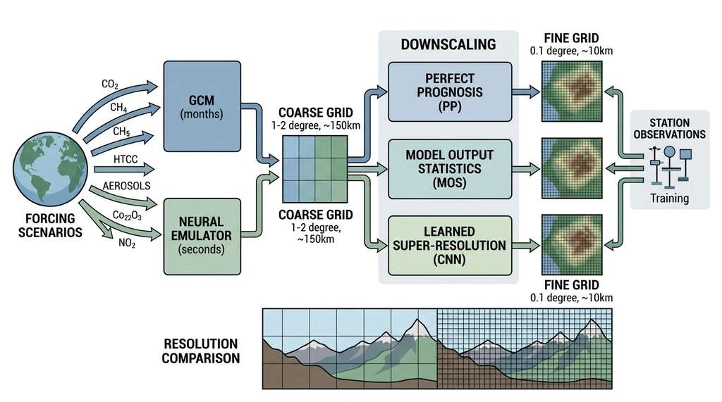
Weather prediction asks "what will happen next week?" Climate science asks "how will the statistical distribution of weather change over decades?" These are fundamentally different questions. A weather model must track individual atmospheric states; a climate model must reproduce the long-term statistics (mean temperature, precipitation patterns, variability, extremes) under different forcing scenarios. General circulation models (GCMs) answer climate questions by running physics-based simulations for centuries, but this costs millions of CPU hours per scenario. Climate emulators learn to approximate GCM outputs from forcing inputs, producing century-long projections in seconds. Downscaling then translates coarse global projections to the fine regional detail that adaptation planning requires. Figure 51.6 illustrates this pipeline from forcing scenarios through emulation and downscaling to local impact assessment.
1. Climate Emulation
In 2023, a team at the University of Leeds reportedly reproduced a century of climate projections from a state-of-the-art general circulation model in under forty seconds on a single GPU, matching the spatial warming patterns to within a fraction of a degree for the specific GCM and scenarios tested. The trick was not a faster supercomputer; it was a neural network trained to skip the physics entirely.
Every degree of global warming triggers cascading decisions: which coastlines to fortify, which crops to replant, which infrastructure to relocate. Policymakers need projections across hundreds of emission scenarios, but each full GCM run can consume weeks of supercomputer time, making exhaustive exploration impossible with physics-based models alone.
What. A climate emulator is a statistical or neural model that maps forcing scenarios (greenhouse gas concentrations, aerosol emissions, land-use changes) to climate response fields (spatial patterns of temperature, precipitation, sea level pressure) without running a physics-based GCM. The emulator learns the input-output relationship of the GCM from a training set of completed simulations.
Why. The Coupled Model Intercomparison Project (CMIP) produces climate projections by running dozens of GCMs under multiple Shared Socioeconomic Pathways (SSPs), where each SSP defines a plausible future trajectory of emissions, land use, and socioeconomic development. Each combination of model and scenario costs weeks to months of supercomputer time. Policy analysis, uncertainty quantification, and rapid scenario exploration all benefit from emulators that can produce comparable projections in seconds.
How. The simplest emulators use pattern scaling: assume that the spatial pattern of warming is constant and only the global mean temperature changes with forcing. More sophisticated approaches use Gaussian processes, random forests, or neural networks to learn non-linear relationships between forcing and spatial response patterns. Figure 51.2.1 illustrates climate emulation and downscaling pipeline.
Pattern Scaling in Detail
Pattern scaling starts with a GCM run that produces a spatial warming map for one reference scenario. The method then normalizes that map by the global mean temperature change, yielding a dimensionless "fingerprint." For any new forcing scenario, it multiplies this fingerprint by the predicted global mean temperature (often from a simple energy balance model). The result is an approximate spatial field produced without re-running the GCM. This matters because it collapses century-long spatial projections to a single scalar prediction problem, cutting compute by orders of magnitude. Pattern scaling works well when forcing changes are moderate and the spatial response scales linearly with global temperature. When strong aerosol forcing, abrupt ice-sheet changes, or precipitation extremes break the linearity assumption, learned emulators or full GCM runs become necessary.
When. Use emulators for scenario screening (which SSPs produce dangerous warming in which regions?), uncertainty quantification (how much does the response vary across GCMs?), and impact assessment (feeding climate projections into agricultural, hydrological, or economic models that need thousands of scenarios). In short: an emulator trades physical fidelity for the ability to ask a thousand "what if" questions in the time a GCM answers one.
Common Misconception
A frequent misconception is that a faster emulator is a better climate model. Speed is an engineering advantage, not a scientific one: the emulator inherits all of the biases, structural assumptions, and domain limitations of the GCM it was trained on. If the training GCM underestimates Arctic amplification or misrepresents monsoon dynamics, the emulator will faithfully reproduce those same errors at a thousand times the speed.
A climate emulator is not a climate model. It does not solve the Navier-Stokes equations (the partial differential equations governing fluid motion in the atmosphere and ocean) or represent cloud microphysics. It learns the mapping that a GCM implements, bypassing the physics entirely. This makes it fast but also means it cannot extrapolate beyond the forcing scenarios it was trained on. If the real climate enters a regime that no GCM has simulated (a sudden ice-sheet collapse, a methane feedback loop), the emulator has no mechanism to capture the new physics. This is why emulators complement rather than replace GCMs: emulators accelerate exploration within the GCM's domain of validity, while GCMs push the boundaries of physical understanding. The same principle applies to the scientific ML surrogates we built in Chapter 33.
"""
Climate emulator: predict spatial temperature response from
forcing scenarios using a neural network trained on CMIP6 output.
"""
import numpy as np
import torch
import torch.nn as nn
import xarray as xr
from pathlib import Path


class ClimateEmulator(nn.Module):
    """Neural climate emulator mapping forcing to spatial response.

    Input: time series of global forcings (CO2, CH4, SO2, etc.)
    Output: spatial temperature anomaly field (lat x lon)

    Architecture: encode the forcing time series with a 1D CNN,
    then decode to spatial patterns with a learned basis.
    """

    def __init__(self, n_forcings: int = 4, n_years: int = 86,
                 n_lat: int = 64, n_lon: int = 128,
                 n_basis: int = 32, hidden_dim: int = 256):
        super().__init__()
        self.n_lat = n_lat
        self.n_lon = n_lon
        self.n_basis = n_basis

        # Temporal encoder: process forcing time series
        self.forcing_encoder = nn.Sequential(
            nn.Conv1d(n_forcings, hidden_dim, kernel_size=5, padding=2),
            nn.ReLU(),
            nn.Conv1d(hidden_dim, hidden_dim, kernel_size=5, padding=2),
            nn.ReLU(),
            nn.AdaptiveAvgPool1d(1),  # global average over time
            nn.Flatten(),
        )

        # Map encoded forcing to basis coefficients
        self.basis_predictor = nn.Sequential(
            nn.Linear(hidden_dim, hidden_dim),
            nn.ReLU(),
            nn.Linear(hidden_dim, n_basis),
        )

        # Learnable spatial basis patterns
        # Each basis pattern is a (lat, lon) field
        self.spatial_basis = nn.Parameter(
            torch.randn(n_basis, n_lat, n_lon) * 0.01
        )

        # Predict per-year scaling from forcing time series
        self.year_predictor = nn.Sequential(
            nn.Conv1d(n_forcings, hidden_dim, kernel_size=5, padding=2),
            nn.ReLU(),
            nn.Conv1d(hidden_dim, n_basis, kernel_size=1),
        )

    def forward(self, forcings: torch.Tensor) -> torch.Tensor:
        """Predict spatial temperature response from forcing scenario.

        Args:
            forcings: (batch, n_forcings, n_years)
                Time series of greenhouse gas concentrations,
                aerosol emissions, etc.
        Returns:
            temperature_anomaly: (batch, n_years, n_lat, n_lon)
                Predicted temperature change relative to baseline
        """
        # Global basis coefficients from forcing summary
        encoded = self.forcing_encoder(forcings)   # (B, hidden)
        global_coeff = self.basis_predictor(encoded)  # (B, n_basis)

        # Per-year modulation of basis coefficients
        year_coeff = self.year_predictor(forcings)  # (B, n_basis, n_years)

        # Combine: global pattern x yearly modulation
        coeff = global_coeff.unsqueeze(-1) * year_coeff  # (B, n_basis, years)

        # Reconstruct spatial field from basis
        # spatial_basis: (n_basis, lat, lon) -> (1, n_basis, lat*lon)
        basis_flat = self.spatial_basis.reshape(self.n_basis, -1).unsqueeze(0)

        # coeff: (B, n_basis, years) @ basis: (1, n_basis, lat*lon)
        # -> (B, years, lat*lon)
        response = torch.einsum("bkt,bkp->btp", coeff.transpose(1, 2),
                                basis_flat.expand(coeff.shape[0], -1, -1))

        return response.reshape(-1, coeff.shape[-1],
                                self.n_lat, self.n_lon)


def train_emulator(model: ClimateEmulator,
                   forcing_data: torch.Tensor,
                   target_data: torch.Tensor,
                   n_epochs: int = 200,
                   lr: float = 1e-3) -> list[float]:
    """Train the climate emulator on CMIP6 model output.

    The training set consists of multiple GCM simulations
    under different SSP scenarios. Each sample is a
    (forcing_timeseries, temperature_response) pair.

    Args:
        model: ClimateEmulator instance
        forcing_data: (n_scenarios, n_forcings, n_years)
        target_data: (n_scenarios, n_years, n_lat, n_lon)
        n_epochs: Training epochs
        lr: Learning rate
    Returns:
        List of training losses
    """
    optimizer = torch.optim.AdamW(model.parameters(), lr=lr,
                                  weight_decay=1e-5)
    scheduler = torch.optim.lr_scheduler.CosineAnnealingLR(
        optimizer, T_max=n_epochs
    )
    losses = []

    for epoch in range(n_epochs):
        model.train()
        pred = model(forcing_data)
        loss = nn.functional.mse_loss(pred, target_data)

        # Add spatial smoothness regularization
        # Penalize high-frequency spatial noise
        dx = pred[:, :, :, 1:] - pred[:, :, :, :-1]
        dy = pred[:, :, 1:, :] - pred[:, :, :-1, :]
        smooth_loss = 0.01 * (dx.pow(2).mean() + dy.pow(2).mean())

        total_loss = loss + smooth_loss
        optimizer.zero_grad()
        total_loss.backward()
        optimizer.step()
        scheduler.step()

        losses.append(total_loss.item())
        if (epoch + 1) % 50 == 0:
            print(f"Epoch {epoch+1}/{n_epochs}, "
                  f"MSE: {loss.item():.6f}, "
                  f"Smooth: {smooth_loss.item():.6f}")

return losses2. Statistical Downscaling
GCMs and climate emulators produce projections on coarse grids (typically 1 to 2 degrees, or 100 to 200 km). Adaptation planning needs local detail: how will rainfall change in a specific river catchment? Will a particular city face more extreme heat days? Downscaling bridges this resolution gap.
Statistical downscaling learns relationships between large-scale atmospheric patterns and local weather variables from historical observations. The assumption is that these relationships, calibrated on the recent past, will hold under future climate conditions. This "stationarity assumption" poses the primary limitation of statistical downscaling. If climate change alters local processes (by shifting the jet stream or changing land surface properties), the learned relationships break down.
Mental Model
Think of statistical downscaling like a local weather forecaster who has spent decades learning that "when the barometric pressure drops and the wind shifts southwest, our valley gets heavy rain." She does not simulate the physics of the atmosphere; she recognizes recurring large-scale patterns and translates them into local consequences based on years of observed correlation. If the climate shifts so that entirely new wind patterns appear (ones she has never seen before), her local translation rules stop working. That is exactly the stationarity assumption: the forecaster's learned dictionary of "large pattern maps to local outcome" remains valid only as long as the large-scale regimes stay within the range she trained on.
Three families of methods dominate.
Perfect prognosis (PP) methods train a regression model from observed large-scale predictors (reanalysis data, where reanalysis is a retrospective atmospheric reconstruction that blends observations with a weather model to produce a spatially complete, physically consistent record of past weather) to observed local-scale predictands (the target variables being predicted, such as station-level temperature or precipitation). At prediction time, the GCM's large-scale output replaces the reanalysis data. This assumes that the GCM represents large-scale patterns well enough to substitute for reanalysis.
Model output statistics (MOS) methods train directly on GCM output paired with observations, learning to correct the GCM's biases. MOS is simpler but couples the downscaling model to a specific GCM.
Learned downscaling uses convolutional neural networks or diffusion models to super-resolve coarse climate fields, treating the problem as analogous to image super-resolution. This approach has the advantage of producing spatially coherent high-resolution fields rather than point predictions.
"""
Statistical downscaling: from coarse GCM output to fine-resolution
local climate using both classical and neural approaches.
"""
import numpy as np
import torch
import torch.nn as nn
import xarray as xr
from sklearn.linear_model import Ridge
from sklearn.preprocessing import StandardScaler


class PerfectPrognosisDownscaler:
    """Classical statistical downscaling via perfect prognosis.

    Trains a Ridge regression from large-scale reanalysis
    predictors to local station observations. At inference time,
    GCM output replaces reanalysis as input.
    """

    def __init__(self, alpha: float = 1.0):
        self.scaler_X = StandardScaler()
        self.scaler_y = StandardScaler()
        self.model = Ridge(alpha=alpha)

    def fit(self, predictors: np.ndarray,
            targets: np.ndarray) -> "PerfectPrognosisDownscaler":
        """Train on reanalysis predictors and station observations.

        Args:
            predictors: (n_samples, n_features) large-scale fields
                (e.g., 500hPa geopotential, 850hPa temperature,
                sea level pressure) extracted from ERA5
            targets: (n_samples,) local variable
                (e.g., daily max temperature at a station)
        Returns:
            self
        """
        X = self.scaler_X.fit_transform(predictors)
        y = self.scaler_y.fit_transform(targets.reshape(-1, 1)).ravel()
        self.model.fit(X, y)
        return self

    def predict(self, gcm_predictors: np.ndarray) -> np.ndarray:
        """Downscale GCM output to local predictions.

        Args:
            gcm_predictors: (n_samples, n_features) large-scale
                fields from a GCM simulation
        Returns:
            Local-scale predictions
        """
        X = self.scaler_X.transform(gcm_predictors)
        y_scaled = self.model.predict(X)
        return self.scaler_y.inverse_transform(
            y_scaled.reshape(-1, 1)
        ).ravel()


class ConvDownscaler(nn.Module):
    """Neural downscaling via learned super-resolution.

    Treats climate downscaling as a super-resolution problem:
    upscale coarse (e.g., 1-degree) fields to fine resolution
    (e.g., 0.1-degree) using residual convolutional blocks and
    pixel shuffle upsampling.

    This produces spatially coherent high-resolution fields
    rather than independent point predictions.
    """

    def __init__(self, in_channels: int = 5, scale_factor: int = 10,
                 hidden_channels: int = 64, n_res_blocks: int = 8):
        super().__init__()
        self.scale_factor = scale_factor

        # Initial feature extraction
        self.head = nn.Sequential(
            nn.Conv2d(in_channels, hidden_channels, 3, padding=1),
            nn.ReLU(),
        )

        # Residual blocks for deep feature extraction
        self.body = nn.Sequential(*[
            ResidualBlock(hidden_channels) for _ in range(n_res_blocks)
        ])

        # Upsampling via sub-pixel convolution (pixel shuffle)
        upsample_layers = []
        remaining = scale_factor
        while remaining > 1:
            if remaining >= 5:
                factor = 5
            elif remaining >= 2:
                factor = 2
            else:
                factor = remaining
            upsample_layers.extend([
                nn.Conv2d(hidden_channels,
                          hidden_channels * factor ** 2, 3, padding=1),
                nn.PixelShuffle(factor),
                nn.ReLU(),
            ])
            remaining //= factor

        self.upsample = nn.Sequential(*upsample_layers)

        # Final output layer
        self.tail = nn.Conv2d(hidden_channels, 1, 3, padding=1)

    def forward(self, coarse: torch.Tensor,
                topography: torch.Tensor = None) -> torch.Tensor:
        """Downscale coarse climate field to fine resolution.

        Args:
            coarse: (batch, in_channels, lat_coarse, lon_coarse)
                Coarse-resolution fields (temperature, pressure,
                humidity, wind components)
            topography: Optional (batch, 1, lat_fine, lon_fine)
                High-resolution topography for conditioning
        Returns:
            fine: (batch, 1, lat_fine, lon_fine) downscaled field
        """
        x = self.head(coarse)
        x = x + self.body(x)  # global skip connection
        x = self.upsample(x)
        x = self.tail(x)

        # Add topographic correction if available
        if topography is not None:
            # Lapse rate correction: temperature decreases with altitude
            lapse_rate = -6.5e-3  # K/m, standard atmosphere
            x = x + lapse_rate * topography

        return x


class ResidualBlock(nn.Module):
    """Residual convolutional block with batch normalization."""

    def __init__(self, channels: int):
        super().__init__()
        self.block = nn.Sequential(
            nn.Conv2d(channels, channels, 3, padding=1),
            nn.BatchNorm2d(channels),
            nn.ReLU(),
            nn.Conv2d(channels, channels, 3, padding=1),
            nn.BatchNorm2d(channels),
        )

    def forward(self, x):
return x + self.block(x)A European climate adaptation project needed 0.1-degree precipitation projections for flood risk modeling across Alpine river catchments. Coarse CMIP6 models at 1-degree resolution could not resolve the orographic enhancement (mountains forcing air upward, causing intense local rainfall) that drives Alpine flood risk. The project trained a ConvDownscaler on ERA5 reanalysis paired with high-resolution E-OBS station observations, incorporating a 90-meter digital elevation model (DEM) as a conditioning input. The downscaled projections captured orographic precipitation patterns that the coarse models missed entirely, enabling the first catchment-scale flood risk assessments under SSP2-4.5 and SSP5-8.5 scenarios. The key lesson: topographic conditioning is essential for precipitation downscaling in mountainous terrain.
3. Foundation Models for Earth Observation
Downscaling refines climate projections to local resolution, but those projections are only as useful as the observational data they connect to on the ground, and that ground truth increasingly arrives from space.
Earth observation satellites generate petabytes of multispectral imagery annually; Sentinel-2 alone produces 1.6 TB per day, more raw data every week than the entire Landsat archive accumulated over its first two decades. Traditional pipelines require hand-engineered features and a separate model for every task. Foundation models instead learn general-purpose representations from unlabeled imagery, then adapt with minimal labeled data.
The approach mirrors the foundation model paradigm from Chapter 27: pretrain a large model on self-supervised objectives (masked image modeling, temporal prediction), then fine-tune on downstream tasks. Three models define the current landscape.
Prithvi (IBM/NASA, 2023) is a vision Transformer pretrained on Harmonized Landsat Sentinel-2 (HLS) data. It processes multi-temporal, multi-spectral inputs and has been fine-tuned for flood mapping, wildfire scar detection, and multi-temporal crop segmentation. (As of 2024, Prithvi-2 extends the original with higher resolution, additional sensor modalities, and improved temporal encoding, supporting a broader range of geospatial tasks.)
Clay (Clay Foundation, 2024) trains on diverse satellite modalities (optical, synthetic aperture radar (SAR), DEM) with a masked autoencoder objective, producing embeddings that transfer across sensors and geographies.
SatMAE (Cong et al., 2022) adapts the Masked Autoencoder framework to multispectral satellite imagery, learning to reconstruct masked patches across spectral bands and time steps. (As of 2025, several successors, including SatMAE++ and SpectralGPT, have extended this approach with cross-sensor transfer and spectral-spatial joint pretraining, reflecting rapid progress in the earth observation foundation model space.)
Checkpoint
So far: foundation models for earth observation (Prithvi, Clay, SatMAE) learn general-purpose representations from unlabeled satellite imagery via self-supervised pretraining, then adapt to downstream tasks (flood mapping, crop segmentation, land cover classification) with minimal labeled data, following the same pretrain-then-fine-tune paradigm introduced in Chapter 27.
"""
Using Google Earth Engine for large-scale earth observation
data access and preprocessing, feeding into foundation models.
"""
import ee
import numpy as np
import xarray as xr

# Initialize Earth Engine (requires authentication)
# ee.Authenticate()
# ee.Initialize(project='your-project-id')


def get_ndvi_timeseries(
    geometry: ee.Geometry,
    start_date: str,
    end_date: str,
    cloud_threshold: float = 20.0,
) -> ee.ImageCollection:
    """Extract cloud-filtered NDVI time series from Sentinel-2.

    Normalized Difference Vegetation Index (NDVI) tracks
    vegetation health and phenology from space:
    NDVI = (NIR - Red) / (NIR + Red)

    Args:
        geometry: Region of interest as an Earth Engine geometry
        start_date: Start date (YYYY-MM-DD)
        end_date: End date (YYYY-MM-DD)
        cloud_threshold: Maximum cloud cover percentage
    Returns:
        ImageCollection of NDVI images
    """
    s2 = (
        ee.ImageCollection("COPERNICUS/S2_SR_HARMONIZED")
        .filterBounds(geometry)
        .filterDate(start_date, end_date)
        .filter(ee.Filter.lt("CLOUDY_PIXEL_PERCENTAGE",
                             cloud_threshold))
    )

    def add_ndvi(image):
        ndvi = image.normalizedDifference(["B8", "B4"]).rename("NDVI")
        return image.addBands(ndvi)

    return s2.map(add_ndvi).select("NDVI")


def compute_land_surface_temperature(
    geometry: ee.Geometry,
    start_date: str,
    end_date: str,
) -> ee.Image:
    """Compute mean land surface temperature from MODIS.

    Land surface temperature (LST) from the MODIS satellite
    provides a direct measure of surface energy balance,
    critical for urban heat island studies and agriculture.

    Args:
        geometry: Region of interest
        start_date: Start date (YYYY-MM-DD)
        end_date: End date (YYYY-MM-DD)
    Returns:
        Mean LST image in Celsius
    """
    lst = (
        ee.ImageCollection("MODIS/061/MOD11A2")
        .filterBounds(geometry)
        .filterDate(start_date, end_date)
        .select("LST_Day_1km")
    )

    # Convert from scaled integer to Celsius
    mean_lst = lst.mean().multiply(0.02).subtract(273.15)
    return mean_lst.clip(geometry)


def carbon_stock_estimation(
    geometry: ee.Geometry,
    year: int = 2023,
) -> dict:
    """Estimate above-ground carbon stocks using satellite data.

    Combines Global Forest Canopy Height (GEDI/Landsat),
    land cover classification, and allometric models (which
    estimate whole-tree biomass from measurable quantities
    like canopy height using species-specific power-law
    relationships) to estimate carbon stored in vegetation.

    Args:
        geometry: Region of interest
        year: Target year
    Returns:
        Dictionary with area and carbon estimates
    """
    # Global forest canopy height from GEDI/Landsat
    canopy_height = ee.Image(
        "users/nlang/ETH_GlobalCanopyHeight_2020_10m_v1"
    ).clip(geometry)

    # Simple allometric model: biomass ~ height^2.5
    # (Real applications use species-specific allometrics)
    biomass_density = canopy_height.pow(2.5).multiply(0.5)

    # Carbon is approximately 50% of dry biomass
    carbon_density = biomass_density.multiply(0.5)  # tonnes C / ha

    # Compute zonal statistics
    stats = carbon_density.reduceRegion(
        reducer=ee.Reducer.mean().combine(
            ee.Reducer.sum(), sharedInputs=True
        ),
        geometry=geometry,
        scale=30,
        maxPixels=1e9,
    )

    return {
        "mean_carbon_density_tC_per_ha": stats.get("b1_mean"),
        "total_carbon_tC": stats.get("b1_sum"),
        "area_ha": geometry.area().divide(10000),
}4. Carbon Accounting with Satellite Data
The same satellite imagery and foundation model representations that power land cover classification and crop monitoring also enable a more consequential application: tracking the carbon that drives the climate projections we have been emulating and downscaling.
Carbon accounting quantifies greenhouse gas sources, sinks, and stocks across landscapes. Satellite observations provide three complementary measurements. First, atmospheric CO2 concentrations from the Orbiting Carbon Observatory missions (OCO-2/OCO-3) reveal spatial patterns of carbon sources and sinks at regional scale. Second, land cover change from Landsat/Sentinel-2 tracks deforestation, reforestation, and land-use transitions. Third, biomass estimation from Global Ecosystem Dynamics Investigation (GEDI) lidar (light detection and ranging, which measures surface structure by timing laser pulse reflections) and SAR (Sentinel-1) quantifies the carbon stored in vegetation.
AI enters carbon accounting in two ways. Machine learning models fuse these heterogeneous data sources into consistent carbon flux estimates (how much CO2 is entering or leaving each grid cell). And foundation models pretrained on satellite imagery can classify land cover, detect disturbances, and estimate biomass with far less labeled training data than traditional approaches.
"""
Zarr-based climate data pipeline with the Pangeo stack.
Demonstrates cloud-native access to analysis-ready climate data.
"""
import xarray as xr
import numpy as np
import dask


def load_era5_from_zarr(
    variable: str = "2m_temperature",
    time_range: tuple[str, str] = ("2020-01-01", "2020-12-31"),
    region: dict = None,
) -> xr.DataArray:
    """Load ERA5 reanalysis data from cloud-hosted Zarr store.

    ERA5 is ECMWF's fifth-generation global atmospheric
    reanalysis, covering 1940 to the present at 0.25-degree
    resolution. The Pangeo ecosystem hosts ERA5 data in Zarr
    format on Google Cloud Storage, enabling lazy loading of
    multi-terabyte datasets without downloading anything to
    local disk.

    Args:
        variable: ERA5 variable name
        time_range: (start, end) date strings
        region: Optional dict with lat/lon bounds
            e.g., {"lat": slice(60, 30), "lon": slice(-10, 40)}
    Returns:
        Lazy-loaded xarray DataArray backed by Dask
    """
    # Cloud-hosted ERA5 in Zarr format (Pangeo)
    store = "gs://gcp-public-data-arco-era5/ar/full_37-1h-0p25deg-chunk-1.zarr-v3"

    ds = xr.open_zarr(store, chunks="auto")
    da = ds[variable].sel(time=slice(*time_range))

    if region:
        da = da.sel(**region)

    return da


def compute_climatology(da: xr.DataArray,
                        baseline: tuple[str, str] = ("1991", "2020")
                        ) -> xr.DataArray:
    """Compute day-of-year climatology over a baseline period.

    The climatology is the expected value for each calendar day,
    used as the reference for anomaly calculations and as a
    baseline forecast in WeatherBench2 evaluations.

    Args:
        da: Input DataArray with a time dimension
        baseline: (start_year, end_year) for the baseline period
    Returns:
        Climatology indexed by day-of-year (1 to 366)
    """
    baseline_data = da.sel(
        time=slice(baseline[0], baseline[1])
    )
    climatology = baseline_data.groupby("time.dayofyear").mean("time")
    return climatology


def compute_anomaly(da: xr.DataArray,
                    climatology: xr.DataArray) -> xr.DataArray:
    """Compute anomaly relative to day-of-year climatology.

    Anomalies are departures from the expected seasonal cycle.
    They isolate the weather signal from the climatological
    background, making it easier to detect trends, extreme
    events, and teleconnection patterns (where teleconnections
    are statistical links between weather anomalies at widely
    separated locations, such as the El Nino/Southern Oscillation
    connecting tropical Pacific sea surface temperatures to
    rainfall patterns across multiple continents).

    Args:
        da: Input DataArray
        climatology: Day-of-year climatology from compute_climatology
    Returns:
        Anomaly DataArray
    """
    return da.groupby("time.dayofyear") - climatology


def spatial_average(da: xr.DataArray,
                    weights: xr.DataArray = None) -> xr.DataArray:
    """Area-weighted spatial average.

    Without area weighting, a naive average over a regular
    lat-lon grid overweights polar regions where grid cells
    have less physical area.

    Args:
        da: Input DataArray with lat/lon dimensions
        weights: Optional weights; defaults to cos(lat)
    Returns:
        Spatially averaged time series
    """
    if weights is None:
        weights = np.cos(np.deg2rad(da.lat))
        weights = weights / weights.sum()

    weighted = da.weighted(weights)
return weighted.mean(["lat", "lon"])The code above builds climate analysis primitives from scratch, but the Pangeo ecosystem provides production-ready alternatives. xarray handles labeled multidimensional arrays with built-in groupby, resampling, and weighted operations. zarr enables chunked, compressed, cloud-native storage. dask parallelizes computations transparently across cores or clusters. intake-esm provides a catalog interface for discovering CMIP6 and other climate datasets. xesmf wraps the ESMF regridding library for conservative interpolation between grids. climpred provides forecast verification metrics. Together, these libraries reduce the pipeline above from dozens of lines to a few configuration calls, while handling edge cases (calendar types, missing data, grid singularities) that production code must address. What took 80 lines here is about 10 lines with the full Pangeo stack.
5. ClimateBench: Evaluating Emulators
With emulators, downscalers, foundation models, and carbon pipelines all competing for adoption, a natural question arises: how do we know which emulator to trust?
ClimateBench (Watson-Parris et al., 2022) provides a standardized evaluation framework for climate emulators, analogous to WeatherBench2 for weather models. The benchmark defines four forcing scenarios (historical + SSP1-2.6, SSP2-4.5, SSP3-7.0, SSP5-8.5) and evaluates emulators on their ability to reproduce the spatial patterns of temperature and precipitation response from NorESM2 (a Norwegian Earth System Model contributing to CMIP6) GCM simulations.
The primary metrics are the normalized global RMSE (NRMSE, where RMSE is the root mean square error across all grid cells) for spatial pattern fidelity and the global mean bias for overall calibration. A good emulator captures both the large-scale pattern (warming amplification over land, Arctic amplification, wet-get-wetter/dry-get-drier precipitation) and the regional detail (the North Atlantic warming hole, the Southern Ocean delay).
"""
ClimateBench-style evaluation for climate emulators.
"""
import numpy as np
import xarray as xr


def normalized_global_rmse(
    predicted: xr.DataArray,
    target: xr.DataArray,
    lat: xr.DataArray = None,
) -> float:
    """Normalized global RMSE for spatial pattern evaluation.

    Normalizes by the spatial standard deviation of the target
    field, so NRMSE = 1.0 means the emulator's error is as
    large as the signal's spatial variability.

    Args:
        predicted: Emulated spatial field
        target: GCM target spatial field
        lat: Latitude array for area weighting
    Returns:
        NRMSE score (lower is better, 0 = perfect)
    """
    if lat is None:
        lat = predicted.lat

    weights = np.cos(np.deg2rad(lat))
    weights = weights / weights.sum()
    weights_da = xr.DataArray(weights, dims=["lat"],
                              coords={"lat": lat})

    # Weighted RMSE
    sq_error = (predicted - target) ** 2
    wmse = float((sq_error * weights_da).sum(["lat", "lon"])
                 / weights_da.sum())
    rmse = np.sqrt(wmse)

    # Normalize by target spatial standard deviation
    target_var = float(
        ((target - (target * weights_da).sum(["lat", "lon"])) ** 2
         * weights_da).sum(["lat", "lon"])
    )
    target_std = np.sqrt(target_var)

    return rmse / (target_std + 1e-10)


def pattern_correlation(
    predicted: xr.DataArray,
    target: xr.DataArray,
) -> float:
    """Spatial pattern correlation coefficient.

    Measures whether the emulator reproduces the spatial
    structure of the climate response, regardless of amplitude.

    Args:
        predicted: Emulated spatial field
        target: GCM target spatial field
    Returns:
        Correlation coefficient (-1 to 1, higher is better)
    """
    weights = np.cos(np.deg2rad(predicted.lat))

    p_anom = predicted - float((predicted * weights).sum()
                               / weights.sum())
    t_anom = target - float((target * weights).sum()
                            / weights.sum())

    numerator = float((p_anom * t_anom * weights).sum())
    denom = np.sqrt(
        float((p_anom ** 2 * weights).sum())
        * float((t_anom ** 2 * weights).sum())
    )
return numerator / (denom + 1e-10)The IPCC's Working Group I evaluates climate projections across dozens of models and scenarios. Running all combinations with full GCMs is computationally prohibitive. Climate emulators trained on the CMIP6 multi-model ensemble enable rapid screening: given a new emissions pathway, the emulator produces spatial temperature and precipitation projections in seconds, along with inter-model uncertainty ranges. This allows policy-relevant questions ("What is the probability that warming exceeds 2C over South Asia under this pathway?") to be answered in real time during negotiations, rather than requiring months of supercomputer allocation.
Research Frontier
ACE2 (Watt-Meyer et al., 2024, "ACE2: Accurately Learning the Earth's Climatic Variables in a Fully Coupled Global AI Framework") demonstrated the first fully coupled global AI climate model capable of producing stable, physically consistent multi-decade simulations. Unlike emulators that learn a single GCM's input-output mapping, ACE2 autoregressively steps the full atmospheric state forward in time, coupled to a slab ocean model (a simplified ocean representation that treats the ocean as a single mixed layer of fixed depth, exchanging heat with the atmosphere but omitting deep-ocean circulation). Trained on ERA5 reanalysis and AMIP-style runs, ACE2 reproduces realistic climatology, interannual variability, and the spatial structure of warming under increased CO2, all while running roughly 100 times faster than a comparable GCM. This pushes beyond the emulation paradigm covered in this section: rather than approximating a GCM's outputs, ACE2 replaces the GCM's dynamical core entirely with a learned model, raising questions about whether future climate projections can be produced without traditional numerical solvers.
Try It: Build a Pattern-Scaling Emulator from CMIP6 Data
1. Install the required libraries (pip install xarray zarr intake-esm matplotlib numpy) and use intake-esm to load a CMIP6 dataset: search the Pangeo CMIP6 catalog for the NorESM2-LM model, historical experiment, surface air temperature variable (tas), and one ensemble member. Load the data lazily with xr.open_zarr.
2. Compute a baseline climatology (1981 to 2010 mean) and subtract it from the full time series to get annual-mean temperature anomalies on the model's native grid. Also load the corresponding SSP2-4.5 run for the same model.
3. For each year in the historical and SSP2-4.5 records, compute the global-mean temperature anomaly (area-weighted using cos(latitude)) and the corresponding spatial anomaly field. Divide each spatial field by its global mean to obtain dimensionless "fingerprint" patterns.
4. Average all fingerprint patterns across years to get a single mean fingerprint. Multiply this fingerprint by an arbitrary global-mean trajectory (for example, a linear ramp from 0 to 4 K) to produce a synthetic spatial projection. Plot the result on a map using matplotlib with a diverging colormap.
5. Evaluate your pattern-scaling emulator against the actual SSP2-4.5 spatial field: compute the NRMSE and pattern correlation using the functions from Figure 51.11. Observe where pattern scaling succeeds (land/ocean contrast, Arctic amplification) and where it fails (precipitation, regional aerosol effects).
Exercise 51.2.1
A climate emulator trained on CMIP6 produces a spatial temperature fingerprint \(F(x,y)\) normalized so that its area-weighted global mean equals 1.0. Under SSP2-4.5, an energy balance model predicts a global mean warming of 2.3 K by 2100. Using pattern scaling, what is the predicted local warming at a grid cell where \(F(x,y) = 1.8\)? Now suppose the same grid cell shows 3.1 K of warming in the actual GCM run. What is the pattern-scaling error at that grid cell, and what physical process might explain why pattern scaling underestimates the response there?
Hint
Pattern scaling predicts local warming as \(\Delta T_{\text{local}} = F(x,y) \times \Delta T_{\text{global}}\). For the second part, consider locations where local feedbacks (such as snow/ice albedo feedback or soil moisture depletion) amplify warming beyond what a static fingerprint captures.
Step-Through: Pattern Scaling with a 2x2 Grid
Trace through pattern scaling on a tiny 2x2 latitude-longitude grid. Suppose a GCM reference run under a +1 K global mean warming produces the following spatial temperature anomalies (in K):
Grid cell (60N, 0E): 1.6 K | Grid cell (60N, 90E): 1.2 K
Grid cell (30N, 0E): 0.8 K | Grid cell (30N, 90E): 0.4 K
Step 1 (Normalize): Compute the area-weighted global mean. Weights are \(\cos(60°) = 0.5\) for the top row and \(\cos(30°) = 0.866\) for the bottom row. Weighted mean = \((0.5 \times (1.6 + 1.2) + 0.866 \times (0.8 + 0.4)) / (2 \times 0.5 + 2 \times 0.866)\) = \((1.4 + 1.0392) / 2.732\) = \(0.893\) K.
Step 2 (Fingerprint): Divide each cell by 0.893 to get \(F\): (60N,0E) = 1.79, (60N,90E) = 1.34, (30N,0E) = 0.90, (30N,90E) = 0.45.
Step 3 (Project): For a new scenario with \(\Delta T_{\text{global}} = 3.0\) K, multiply: (60N,0E) = 5.37 K, (60N,90E) = 4.03 K, (30N,0E) = 2.69 K, (30N,90E) = 1.34 K. The Arctic amplification pattern (top row warming more) is preserved at any global mean, which is exactly the strength and the limitation of the method.
Real-World Application: ClimateTrace Global Emissions Monitoring
Climate TRACE (launched 2021) combines satellite imagery, remote sensing, and ML models to independently monitor greenhouse gas emissions from over 80,000 individual facilities worldwide, including power plants, steel mills, and oil fields. The system uses foundation-model-derived features from Sentinel-2 and Landsat imagery, paired with atmospheric observations from OCO-2 and the TROPOspheric Monitoring Instrument (TROPOMI), to estimate facility-level CO2 and methane emissions without relying on self-reported data. This satellite-based accounting has in several cases indicated that actual emissions from some countries and sectors may be 50 to 100 percent higher than officially reported figures. (As of 2025, Climate TRACE tracks over 350 million assets across all major sectors and countries, and its data feeds directly into the Global Stocktake process under the Paris Agreement.)
The Fastest Climate Model Runs on a Spreadsheet
Before neural emulators existed, the most widely used "fast climate model" was MAGICC (Model for the Assessment of Greenhouse gas Induced Climate Change), first written in 1987. MAGICC is essentially a box model: it represents the entire ocean as a handful of thermal reservoirs connected by diffusion, the atmosphere as a single layer, and the carbon cycle as a few coupled differential equations. Despite this radical simplification, MAGICC has been used in every IPCC assessment report since 1990 to translate emissions scenarios into global temperature projections. Its predictions have generally tracked the actual observed warming to within a few tenths of a degree, though its skill at regional scales and for non-temperature variables is more limited. The lesson: for global mean temperature, a well-calibrated simple model can outperform a poorly calibrated complex one, a theme that recurs whenever we compare emulators to their parent GCMs.
Lab: Train and Evaluate a Minimal Climate Emulator
Goal: Build a pattern-scaling emulator from publicly available CMIP6 data and measure its accuracy against a held-out scenario.
Tools needed: Python 3.10+, xarray, zarr, intake-esm, numpy, matplotlib (install via pip install xarray zarr intake-esm numpy matplotlib).
Procedure (25 minutes):
1. Use intake-esm to load the Pangeo CMIP6 catalog and retrieve surface air temperature (tas) from the NorESM2-LM model for the historical run and two SSP scenarios (SSP2-4.5 and SSP5-8.5). Compute annual means and a 1981 to 2010 baseline climatology.
2. Using the historical run, compute the area-weighted global mean anomaly for each year and divide each spatial field by it to produce yearly fingerprints. Average these into a single mean fingerprint.
3. Hold out SSP5-8.5 as your test set. Predict its spatial warming by multiplying your fingerprint by the SSP5-8.5 global mean trajectory. Compute the NRMSE and pattern correlation against the actual GCM spatial fields.
What to vary: Try building separate fingerprints for land and ocean cells, or for different latitude bands. Try using SSP2-4.5 instead of the historical run to derive the fingerprint.
What to observe: Where does pattern scaling work well (temperature over mid-latitude land)? Where does it break down (precipitation, polar regions, areas with strong aerosol forcing)? How does the NRMSE change across decades as the forcing grows larger?