51.3 Extreme Events and Attribution

"The heatwave was a one-in-a-thousand-year event. Then it happened again the next summer. I updated my priors, but my confidence intervals filed a formal complaint."

A Return Period Estimate in Need of Recalibration

1. Extreme Value Theory

What. When Houston's 500-year flood struck three years in a row (2015, 2016, 2017), engineers discovered that the statistical model behind the "500-year" label was never designed for a climate in motion. Extreme value theory (EVT) replaces naive tail extrapolation with distributions built specifically for extremes, producing rigorous estimates of return levels (the value expected to be exceeded once in a given period) and return periods (the average recurrence interval for a given extreme) that can track a shifting climate.

Why. Infrastructure, insurance, and adaptation planning need answers to questions like "what is the maximum daily rainfall with a 1% annual probability of being exceeded?" Standard Gaussian assumptions break down in the tails. EVT provides the mathematical framework for these calculations.

How. Two approaches dominate. The block maxima method fits a Generalized Extreme Value (GEV) distribution to annual maxima (e.g., the highest daily temperature each year). The peaks-over-threshold (POT) method fits a Generalized Pareto Distribution (GPD) to all exceedances above a high threshold, using more data and producing better estimates when a reliable threshold exists.

The GEV Distribution

The GEV distribution has three parameters: location \(\mu\), scale \(\sigma > 0\), and shape \(\xi\):

The shape parameter \(\xi\) determines the tail behavior. When \(\xi > 0\) (Frechet type), the tail is heavy; when \(\xi = 0\) (Gumbel type), the tail is exponential; when \(\xi < 0\) (Weibull type), the tail has an upper bound. For temperature extremes, \(\xi\) is typically near zero or slightly negative. For precipitation, \(\xi\) is typically positive, reflecting the heavy-tailed nature of rainfall extremes. In short: the shape of the tail, captured in a single parameter, determines whether extreme events have a hard physical ceiling or can always surprise you with something worse.

"""
Extreme value analysis for climate data:
GEV fitting, return levels, and non-stationary models.
"""
import numpy as np
from scipy import stats
from scipy.optimize import minimize
from dataclasses import dataclass


@dataclass
class GEVFit:
    """Result of a GEV distribution fit."""
    location: float     # mu
    scale: float        # sigma
    shape: float        # xi
    nll: float          # negative log-likelihood
    aic: float          # Akaike Information Criterion


def fit_gev(block_maxima: np.ndarray) -> GEVFit:
    """Fit a Generalized Extreme Value distribution to block maxima.

    Uses maximum likelihood estimation via scipy's genextreme,
    which parameterizes the shape as c = -xi (note the sign
    convention difference from the climate literature).

    Args:
        block_maxima: Array of annual (or seasonal) maxima
    Returns:
        GEVFit with estimated parameters
    """
    # scipy uses c = -xi convention
    c, loc, scale = stats.genextreme.fit(block_maxima)
    xi = -c  # Convert to climate convention

    # Negative log-likelihood for model comparison
    nll = -np.sum(stats.genextreme.logpdf(block_maxima,
                                          c, loc=loc, scale=scale))
    aic = 2 * 3 + 2 * nll  # 3 parameters

    return GEVFit(location=loc, scale=scale, shape=xi,
                  nll=nll, aic=aic)


def return_level(gev: GEVFit, return_period: float) -> float:
    """Compute the return level for a given return period.

    The T-year return level is the value that is exceeded
    once every T years on average.

    Args:
        gev: Fitted GEV parameters
        return_period: Return period in years (e.g., 100)
    Returns:
        Return level value
    """
    p = 1 - 1.0 / return_period
    if abs(gev.shape) < 1e-8:
        # Gumbel case (xi -> 0)
        return gev.location - gev.scale * np.log(-np.log(p))
    else:
        # General GEV case
        yp = -np.log(p)
        return gev.location + gev.scale / gev.shape * (
            yp ** (-gev.shape) - 1
        )


def return_level_confidence(block_maxima: np.ndarray,
                            return_period: float,
                            n_bootstrap: int = 1000,
                            ci: float = 0.95) -> tuple[float, float, float]:
    """Bootstrap confidence interval for return levels.

    Resamples the block maxima, refits the GEV for each
    resample, and computes the return level distribution.

    Args:
        block_maxima: Array of annual maxima
        return_period: Return period in years
        n_bootstrap: Number of bootstrap resamples
        ci: Confidence level
    Returns:
        (lower, median, upper) return level estimates
    """
    rng = np.random.default_rng(42)
    n = len(block_maxima)
    levels = []

    for _ in range(n_bootstrap):
        sample = rng.choice(block_maxima, size=n, replace=True)
        try:
            gev = fit_gev(sample)
            rl = return_level(gev, return_period)
            if np.isfinite(rl):
                levels.append(rl)
        except Exception:
            continue

    levels = np.array(levels)
    alpha = (1 - ci) / 2
    return (
        float(np.quantile(levels, alpha)),
        float(np.median(levels)),
        float(np.quantile(levels, 1 - alpha)),
    )


class NonstationaryGEV:
    """GEV with time-varying location parameter.

    In a changing climate, the distribution of extremes is
    not stationary. The simplest non-stationary model lets
    the location parameter trend linearly with time:
    mu(t) = mu_0 + mu_1 * t

    This captures the shift in extreme value distributions
    due to global warming.
    """

    def __init__(self):
        self.params = None

    def _neg_log_likelihood(self, params: np.ndarray,
                            data: np.ndarray,
                            time: np.ndarray) -> float:
        """Negative log-likelihood for non-stationary GEV.

        Args:
            params: [mu_0, mu_1, log_sigma, xi]
            data: Block maxima values
            time: Normalized time covariate
        Returns:
            Negative log-likelihood
        """
        mu_0, mu_1, log_sigma, xi = params
        sigma = np.exp(log_sigma)
        mu = mu_0 + mu_1 * time

        z = (data - mu) / sigma

        if abs(xi) < 1e-8:
            # Gumbel case
            nll = np.sum(np.log(sigma) + z + np.exp(-z))
        else:
            w = 1 + xi * z
            if np.any(w <= 0):
                return 1e10
            nll = np.sum(
                np.log(sigma)
                + (1 + 1 / xi) * np.log(w)
                + w ** (-1 / xi)
            )

        return nll

    def fit(self, data: np.ndarray,
            time: np.ndarray) -> dict:
        """Fit non-stationary GEV to block maxima with time covariate.

        Args:
            data: Block maxima values
            time: Time covariate (e.g., year - 1950)
        Returns:
            Dictionary with fitted parameters and diagnostics
        """
        # Normalize time to [0, 1]
        t_norm = (time - time.min()) / (time.max() - time.min())

        # Initialize from stationary fit
        gev0 = fit_gev(data)
        x0 = [gev0.location, 0.0, np.log(gev0.scale), gev0.shape]

        result = minimize(
            self._neg_log_likelihood, x0,
            args=(data, t_norm),
            method="Nelder-Mead",
            options={"maxiter": 10000},
        )

        mu_0, mu_1, log_sigma, xi = result.x
        self.params = {
            "mu_0": mu_0, "mu_1": mu_1,
            "sigma": np.exp(log_sigma), "xi": xi,
        }

        return {
            "params": self.params,
            "nll": result.fun,
            "aic": 2 * 4 + 2 * result.fun,
            "trend_per_decade": mu_1 / (time.max() - time.min()) * 10,
            "converged": result.success,
        }

Non-stationarity reshapes how we define "extreme," but real-world disasters rarely stem from a single variable exceeding a threshold; they arise when multiple climate drivers combine in unusual ways.

2. Detecting Extreme Events in Climate Data

Detecting extreme events in high-dimensional climate data goes beyond fitting univariate distributions. A compound event (simultaneous heat and drought, or a tropical cyclone making landfall during a king tide, where a king tide is an exceptionally high astronomical tide caused by the alignment of the sun and moon) may not be extreme in any single variable but is extreme in its combination. Multivariate anomaly detection, building on the methods from Chapter 30, captures these compound extremes.

A compound extreme event occurs when two or more climate variables combine to produce severe impacts, even though neither variable alone qualifies as extreme. These events account for a disproportionate share of climate-related damage. The 2022 Pakistan floods resulted from simultaneous monsoon intensification and upstream glacial melt; neither factor was record-breaking on its own. To detect such events, analysts construct a joint distribution over multiple climate variables (temperature, precipitation, soil moisture, wind speed) and flag observations in the low-probability region of that joint space. This approach outperforms univariate extreme detection whenever impacts depend on co-occurring hazards: coastal flooding (storm surge plus river discharge plus high tide) or crop failure (heat plus drought during a critical growth stage).

"""
Multivariate extreme event detection in climate data.
Combines anomaly detection with spatial clustering to
identify coherent extreme weather events.
"""
import numpy as np
import xarray as xr
from sklearn.decomposition import PCA
from sklearn.ensemble import IsolationForest
from scipy.ndimage import label as ndimage_label
from dataclasses import dataclass, field


@dataclass
class ExtremeEvent:
    """Detected extreme weather event."""
    start_date: str
    end_date: str
    center_lat: float
    center_lon: float
    area_km2: float
    max_anomaly: float
    event_type: str
    spatial_extent: np.ndarray = field(repr=False)


def detect_heatwaves(
    temperature: xr.DataArray,
    climatology: xr.DataArray,
    threshold_percentile: float = 95,
    min_duration_days: int = 3,
    min_area_gridcells: int = 50,
) -> list[ExtremeEvent]:
    """Detect heatwave events using exceedance-duration-area criteria.

    A heatwave is defined as a spatially contiguous region where
    temperature exceeds the local climatological percentile for
    at least a minimum number of consecutive days.

    Args:
        temperature: Daily temperature DataArray (time, lat, lon)
        climatology: Day-of-year climatological percentile
        threshold_percentile: Percentile threshold for exceedance
        min_duration_days: Minimum consecutive exceedance days
        min_area_gridcells: Minimum spatial extent in grid cells
    Returns:
        List of detected ExtremeEvent objects
    """
    # Compute anomaly relative to day-of-year climatology
    anomaly = temperature.groupby("time.dayofyear") - climatology

    # Compute threshold from climatological distribution
    # (using the entire record for the percentile)
    threshold = float(anomaly.quantile(
        threshold_percentile / 100, dim="time"
    ).mean())

    # Binary exceedance field
    exceedance = (anomaly > threshold).values  # (time, lat, lon)

    events = []
    n_times = exceedance.shape[0]

    # Scan for consecutive exceedance periods
    t = 0
    while t < n_times:
        daily_mask = exceedance[t]

        # Label spatially contiguous regions
        labeled, n_features = ndimage_label(daily_mask)

        for region_id in range(1, n_features + 1):
            region_mask = labeled == region_id
            area = region_mask.sum()

            if area < min_area_gridcells:
                continue

            # Check duration: does this region persist?
            duration = 1
            for dt in range(1, n_times - t):
                future_mask = exceedance[t + dt]
                overlap = (region_mask & future_mask).sum()
                if overlap >= area * 0.5:
                    duration += 1
                else:
                    break

            if duration >= min_duration_days:
                # Compute event properties
                lat_idx, lon_idx = np.where(region_mask)
                lats = temperature.lat.values[lat_idx]
                lons = temperature.lon.values[lon_idx]

                max_anom = float(anomaly.values[
                    t:t+duration, region_mask
                ].max())

                # Approximate area in km^2
                dlat = abs(float(np.diff(temperature.lat[:2])))
                dlon = abs(float(np.diff(temperature.lon[:2])))
                mean_lat = np.mean(lats)
                cell_area = (
                    dlat * 111  # km per degree latitude
                    * dlon * 111 * np.cos(np.deg2rad(mean_lat))
                )
                total_area = area * cell_area

                events.append(ExtremeEvent(
                    start_date=str(temperature.time.values[t])[:10],
                    end_date=str(
                        temperature.time.values[t + duration - 1]
                    )[:10],
                    center_lat=float(np.mean(lats)),
                    center_lon=float(np.mean(lons)),
                    area_km2=float(total_area),
                    max_anomaly=max_anom,
                    event_type="heatwave",
                    spatial_extent=region_mask,
                ))

        t += max(1, duration if events else 1)

    return events


def compound_event_detection(
    variables: dict[str, xr.DataArray],
    n_components: int = 10,
    contamination: float = 0.01,
) -> np.ndarray:
    """Detect compound extreme events using multivariate anomaly detection.

    Compound events are extreme in their combination of variables
    (e.g., simultaneous heat and drought) even when no single
    variable is individually extreme.

    Uses PCA for dimensionality reduction followed by Isolation
    Forest for anomaly scoring.

    Args:
        variables: Dictionary mapping variable names to DataArrays
            (all must share the same time dimension)
        n_components: Number of PCA components to retain
        contamination: Expected fraction of anomalous samples
    Returns:
        anomaly_scores: Array of anomaly scores per time step
            (more negative = more anomalous)
    """
    # Stack variables into a feature matrix
    features = []
    for name, da in variables.items():
        # Spatial average (or could use grid-point features)
        weights = np.cos(np.deg2rad(da.lat))
        spatial_mean = da.weighted(weights).mean(["lat", "lon"])
        features.append(spatial_mean.values)

    X = np.column_stack(features)

    # Standardize
    X = (X - X.mean(axis=0)) / (X.std(axis=0) + 1e-10)

    # PCA for dimensionality reduction
    pca = PCA(n_components=min(n_components, X.shape[1]))
    X_pca = pca.fit_transform(X)

    # Isolation Forest for anomaly detection
    clf = IsolationForest(
        contamination=contamination,
        random_state=42,
        n_estimators=200,
    )
    scores = clf.fit(X_pca).score_samples(X_pca)

    return scores

Detecting that an extreme event occurred is only half the question; the next step is determining whether human activity made it more likely, a challenge that requires separating the fingerprint of anthropogenic forcing from the background noise of natural variability.

3. Optimal Fingerprinting and Detection-Attribution

What. Optimal fingerprinting is the standard statistical framework for detecting and attributing climate change signals. It answers two questions simultaneously. Detection: is the observed climate trend inconsistent with internal variability (where internal variability refers to natural fluctuations generated within the climate system itself, such as El Nino cycles and weather noise, without any change in external forcing) alone? Attribution: what fraction of the observed trend is explained by each forcing agent (greenhouse gases, aerosols, solar variability, volcanic eruptions)?

Why. The IPCC's conclusion that "human influence on the climate system is unequivocal" draws on optimal fingerprinting as one of its central lines of evidence . More practically, attribution science supports climate litigation (proving that a specific entity's emissions contributed to a specific event), adaptation planning (knowing which forcings to mitigate), and loss-and-damage negotiations.

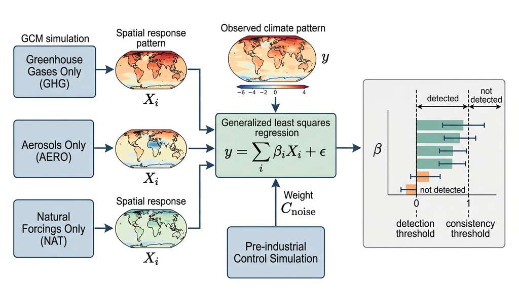
How. Optimal fingerprinting works by regression. The observed climate change pattern \(\mathbf{y}\) is modeled as a linear combination of response patterns \(\mathbf{X}_i\) from individual forcings, plus internal variability noise \(\boldsymbol{\varepsilon}\):

The response patterns \(\mathbf{X}_i\) come from general circulation model (GCM) simulations with individual forcings applied in isolation (greenhouse gases only, aerosols only, natural forcings only). Generalized least squares (a regression method that accounts for correlated, non-uniform noise by weighting observations according to the noise covariance structure) estimates the scaling factors \(\beta_i\), weighting the regression by the covariance of internal variability from pre-industrial control simulations. If \(\beta_i\) is significantly different from zero, the forcing \(i\) is detected. If \(\beta_i\) is consistent with 1.0, the GCM's response to forcing \(i\) is consistent with observations. To keep the regression numerically stable, the data are projected onto leading empirical orthogonal functions (EOFs, the climate science term for PCA eigenvectors; each EOF captures a dominant spatial pattern of variability) , and a residual consistency test (the Allen-Tett test, which checks whether the leftover signal after subtracting all attributed forcings is statistically compatible with internal variability alone) verifies that the model has not missed a significant forcing. Figure 51.3.1 illustrates the optimal fingerprinting detection-attribution framework.

"""
Optimal fingerprinting for detection and attribution
of climate change signals.
"""
import numpy as np
from scipy import linalg
from dataclasses import dataclass


@dataclass
class FingerprintResult:
    """Result of an optimal fingerprinting analysis."""
    scaling_factors: np.ndarray     # beta_i estimates
    confidence_intervals: np.ndarray  # 5-95% CI for each beta
    detected: np.ndarray            # boolean: is beta != 0?
    consistent: np.ndarray          # boolean: is beta consistent with 1?
    residual_consistency: float     # Allen-Tett residual test p-value


def optimal_fingerprinting(
    observations: np.ndarray,
    response_patterns: np.ndarray,
    control_segments: np.ndarray,
    n_eof: int = 10,
    significance_level: float = 0.1,
) -> FingerprintResult:
    """Regularized optimal fingerprinting (Allen & Stott, 2003).

    Detects and attributes climate signals by regressing
    observations onto GCM response patterns for individual forcings
    (greenhouse gases, aerosols, natural), using the covariance of
    internal variability from control simulations as the noise model.

    Args:
        observations: (n_spatial,) observed climate change pattern
            (e.g., temperature trend over 1950-2020, projected
            onto leading EOFs)
        response_patterns: (n_forcings, n_spatial) GCM response
            patterns for each forcing agent (GHG, aerosol, natural)
        control_segments: (n_segments, n_spatial) non-overlapping
            segments of pre-industrial control simulation,
            each the same length as the observational record
        n_eof: Number of EOFs for dimension reduction
        significance_level: Significance level for detection
    Returns:
        FingerprintResult with scaling factors and diagnostics
    """
    n_forcings = response_patterns.shape[0]

    # Step 1: Estimate internal variability covariance from control
    # Split control into two halves: one for regression, one for testing
    n_ctrl = len(control_segments)
    half = n_ctrl // 2
    ctrl_train = control_segments[:half]
    ctrl_test = control_segments[half:]

    # Covariance from training half
    cov_noise = np.cov(ctrl_train.T)

    # Step 2: EOF (empirical orthogonal function) truncation for regularization
    eigenvalues, eigenvectors = linalg.eigh(cov_noise)
    # Sort descending
    idx = np.argsort(eigenvalues)[::-1]
    eigenvalues = eigenvalues[idx[:n_eof]]
    P = eigenvectors[:, idx[:n_eof]]  # (n_spatial, n_eof)

    # Project everything into EOF space
    y = P.T @ observations                         # (n_eof,)
    X = (P.T @ response_patterns.T)                # (n_eof, n_forcings)
    C_inv = np.diag(1.0 / eigenvalues)             # (n_eof, n_eof)

    # Step 3: Generalized least squares
    # beta = (X^T C^{-1} X)^{-1} X^T C^{-1} y
    XtCi = X.T @ C_inv                             # (n_forcings, n_eof)
    fisher = XtCi @ X                              # (n_forcings, n_forcings)
    fisher_inv = linalg.inv(fisher)
    beta = fisher_inv @ XtCi @ y                   # (n_forcings,)

    # Step 4: Confidence intervals from the Fisher information
    beta_var = np.diag(fisher_inv)
    beta_std = np.sqrt(beta_var)

    z_crit = 1.645  # 90% CI (5-95%)
    ci = np.column_stack([
        beta - z_crit * beta_std,
        beta + z_crit * beta_std,
    ])

    # Step 5: Detection test (is beta significantly != 0?)
    detected = ci[:, 0] > 0  # Lower CI bound above zero

    # Step 6: Consistency test (is beta consistent with 1.0?)
    consistent = (ci[:, 0] <= 1.0) & (ci[:, 1] >= 1.0)

    # Step 7: Residual consistency test (Allen-Tett)
    residual = y - X @ beta
    residual_var = float(residual @ C_inv @ residual) / (n_eof - n_forcings)

    # Compare against chi-squared distribution
    from scipy.stats import chi2
    p_value = 1 - chi2.cdf(
        residual_var * (n_eof - n_forcings),
        df=n_eof - n_forcings,
    )

    return FingerprintResult(
        scaling_factors=beta,
        confidence_intervals=ci,
        detected=detected,
        consistent=consistent,
        residual_consistency=float(p_value),
    )


def print_attribution_results(result: FingerprintResult,
                              forcing_names: list[str]) -> None:
    """Print a human-readable attribution summary.

    Args:
        result: FingerprintResult from optimal_fingerprinting
        forcing_names: List of forcing agent names
    """
    print("=" * 60)
    print("OPTIMAL FINGERPRINTING: DETECTION AND ATTRIBUTION")
    print("=" * 60)

    for i, name in enumerate(forcing_names):
        beta = result.scaling_factors[i]
        lo, hi = result.confidence_intervals[i]
        det = "DETECTED" if result.detected[i] else "not detected"
        con = "consistent" if result.consistent[i] else "INCONSISTENT"

        print(f"\n{name}:")
        print(f"  Scaling factor: {beta:.3f} [{lo:.3f}, {hi:.3f}]")
        print(f"  Detection:      {det}")
        print(f"  GCM consistency: {con} with observations")

    print(f"\nResidual test p-value: {result.residual_consistency:.3f}")
    if result.residual_consistency > 0.05:
        print("  Model passes residual consistency test")
    else:
        print("  WARNING: model fails residual consistency test")

4. Event Attribution: The Probabilistic Approach

After every record-breaking disaster, governments and insurers confront the same urgent question: was this just bad luck, or has the climate shifted enough to make such events routine? The answer steers whether billions flow into rebuilding as before or into fundamentally redesigning infrastructure, and it must arrive while the policy window is still open.

While optimal fingerprinting attributes long-term trends, event attribution asks about specific events: "How did climate change alter the probability of this particular heatwave?" The World Weather Attribution (WWA) protocol provides a rigorous framework.

The key quantity is the probability ratio (PR, also called risk ratio or likelihood ratio):

A PR of 5 means the event is five times more likely in the current climate than in a world without human influence. The "factual" climate is the real world with all forcings. The "counterfactual" is a hypothetical world estimated by removing the anthropogenic signal (using GCM simulations with natural forcings only). The event attribution pipeline, illustrated in Figure 51.A, shows how observed extremes flow through factual and counterfactual distribution estimates to produce the probability ratio and fraction of attributable risk.

Mental Model

Think of event attribution like a loaded die. Suppose a standard die has a 1-in-6 chance of rolling a six, but someone has tampered with it so that sixes now come up 5-in-6 of the time. When you roll a six, you cannot point to the weighting and say "83% of this particular roll was caused by the tampering." The roll either happened or it did not. What you can say is that the tampering made sixes five times more likely (probability ratio = 5). The counterfactual climate is the fair die; the factual climate is the loaded one. Attribution quantifies how much the loading shifted the odds, not what fraction of any single roll was "caused" by the weight.

The complementary quantity is the fraction of attributable risk (FAR):

FAR ranges from 0 (no human contribution) to 1 (the event would be impossible without human influence). The 2021 Pacific Northwest heatwave, for example, was assessed by the World Weather Attribution group as "virtually impossible" without climate change (PR > 150, FAR > 0.99) , meaning that in a pre-industrial climate you would wait over 150 lifetimes to see such an event once.

"""
Event attribution: estimate the probability ratio of an
extreme event under factual vs. counterfactual climate.
"""
import numpy as np
from scipy import stats


def estimate_probability_ratio(
    factual_distribution: np.ndarray,
    counterfactual_distribution: np.ndarray,
    threshold: float,
    method: str = "empirical",
) -> dict:
    """Estimate the probability ratio for an extreme event.

    Compares the probability of exceeding a threshold in the
    factual (current) climate vs. the counterfactual (no human
    influence) climate.

    Args:
        factual_distribution: Samples from factual climate
            (from observations or GCM historical simulations)
        counterfactual_distribution: Samples from counterfactual
            (GCM natural-only simulations)
        threshold: Event threshold (e.g., the observed extreme value)
        method: 'empirical' for direct counting,
                'gev' for GEV-based extrapolation
    Returns:
        Dictionary with probability ratio and confidence interval
    """
    if method == "empirical":
        p_factual = np.mean(factual_distribution >= threshold)
        p_counter = np.mean(counterfactual_distribution >= threshold)

    elif method == "gev":
        # Fit GEV to each distribution for better tail estimation
        c_f, loc_f, scale_f = stats.genextreme.fit(factual_distribution)
        c_c, loc_c, scale_c = stats.genextreme.fit(
            counterfactual_distribution
        )
        p_factual = 1 - stats.genextreme.cdf(
            threshold, c_f, loc=loc_f, scale=scale_f
        )
        p_counter = 1 - stats.genextreme.cdf(
            threshold, c_c, loc=loc_c, scale=scale_c
        )

    # Probability ratio
    pr = p_factual / max(p_counter, 1e-10)

    # Fraction of Attributable Risk
    far = 1 - 1 / pr if pr > 1 else 0.0

    # Bootstrap confidence interval for PR
    rng = np.random.default_rng(42)
    n_boot = 1000
    pr_boot = []

    for _ in range(n_boot):
        f_sample = rng.choice(factual_distribution,
                              size=len(factual_distribution),
                              replace=True)
        c_sample = rng.choice(counterfactual_distribution,
                              size=len(counterfactual_distribution),
                              replace=True)

        if method == "empirical":
            pf = np.mean(f_sample >= threshold)
            pc = np.mean(c_sample >= threshold)
        else:
            c_f, loc_f, scale_f = stats.genextreme.fit(f_sample)
            c_c, loc_c, scale_c = stats.genextreme.fit(c_sample)
            pf = 1 - stats.genextreme.cdf(
                threshold, c_f, loc=loc_f, scale=scale_f
            )
            pc = 1 - stats.genextreme.cdf(
                threshold, c_c, loc=loc_c, scale=scale_c
            )

        pr_boot.append(pf / max(pc, 1e-10))

    pr_boot = np.array(pr_boot)

    return {
        "probability_ratio": float(pr),
        "far": float(far),
        "p_factual": float(p_factual),
        "p_counterfactual": float(p_counter),
        "pr_ci_5": float(np.percentile(pr_boot, 5)),
        "pr_ci_95": float(np.percentile(pr_boot, 95)),
        "return_period_factual": 1.0 / max(p_factual, 1e-10),
        "return_period_counterfactual": 1.0 / max(p_counter, 1e-10),
    }


def attribution_summary(result: dict, event_name: str) -> str:
    """Generate a human-readable attribution statement.

    Follows the World Weather Attribution communication format.

    Args:
        result: Output from estimate_probability_ratio
        event_name: Description of the event
    Returns:
        Attribution statement string
    """
    pr = result["probability_ratio"]
    far = result["far"]
    pr_lo = result["pr_ci_5"]
    pr_hi = result["pr_ci_95"]

    lines = [
        f"EVENT ATTRIBUTION: {event_name}",
        "=" * 50,
        f"Probability ratio: {pr:.1f} "
        f"[{pr_lo:.1f} to {pr_hi:.1f}]",
        f"Fraction of attributable risk: {far:.2%}",
        f"Return period (factual climate): "
        f"1-in-{result['return_period_factual']:.0f} years",
        f"Return period (counterfactual): "
        f"1-in-{result['return_period_counterfactual']:.0f} years",
        "",
    ]

    if pr > 100:
        lines.append(
            "CONCLUSION: This event was virtually impossible "
            "without human-caused climate change."
        )
    elif pr > 10:
        lines.append(
            f"CONCLUSION: Climate change made this event "
            f"approximately {pr:.0f} times more likely."
        )
    elif pr > 2:
        lines.append(
            f"CONCLUSION: Climate change approximately "
            f"{'doubled' if pr < 3 else f'increased by {pr:.0f}x'} "
            f"the likelihood of this event."
        )
    elif pr > 1.2:
        lines.append(
            "CONCLUSION: A modest but detectable increase "
            "in likelihood due to climate change."
        )
    else:
        lines.append(
            "CONCLUSION: No significant change in likelihood "
            "attributable to climate change."
        )

    return "\n".join(lines)