Prerequisites
This section builds on the diffusion and flow matching foundations from Section 34.2 and the equivariant architectures from Section 34.3. You should understand the denoising process and how equivariant networks generate 3D structures. Familiarity with policy gradient methods from reinforcement learning is helpful for the REINFORCE material but not required; everything derives from the log-derivative trick, where the gradient of an expectation is rewritten as an expectation of the score function times the reward. The optimization concepts connect to Chapter 45: Optimization for Discovery.
Unconditional generation is rarely useful for discovery. You do not want a random molecule; you want a molecule that binds a specific target, crosses the blood-brain barrier, and can be synthesized in three steps. Conditional generation steers the generative model toward samples with desired properties. Two mechanisms dominate: classifier-free guidance, which biases the diffusion process toward high-property regions during sampling, and REINFORCE, which fine-tunes the generator to maximize a reward function. Both require careful evaluation: did we actually generate good molecules, or did we exploit artifacts in the property predictor? This section covers conditioning, optimization, and the metrics that distinguish genuine discovery from Goodhart's law in action.
1. Classifier-Free Guidance
In practice, training a separate property classifier at every noise level to guide diffusion has proven fragile: the classifier must handle hundreds of noise scales, errors compound across denoising steps, and each new target property requires retraining from scratch. Classifier-free guidance eliminates this entire bottleneck.
Classifier-free guidance (Ho & Salimans, 2022) is the standard method for conditioning diffusion models on target properties without a separate classifier. The idea: train a single model that can operate both conditionally (given a property label \(c\)) and unconditionally (without any label). At sampling time, extrapolate away from the unconditional prediction toward the conditional prediction:
$$\hat{\epsilon}_\theta(x_t, t, c) = \epsilon_\theta(x_t, t, \varnothing) + w \cdot [\epsilon_\theta(x_t, t, c) - \epsilon_\theta(x_t, t, \varnothing)]$$where \(w > 1\) is the guidance scale and \(\varnothing\) denotes the null condition (the unconditional model). When \(w = 1\), this reduces to standard conditional generation. When \(w > 1\), the guidance pushes the model further toward the conditional prediction. The resulting samples match the condition more strongly but lose diversity.
Classifier-free guidance avoids training a separate classifier or property predictor on noisy intermediate states. That per-noise-level approach is brittle and computationally expensive. The mechanism works by jointly training conditional and unconditional pathways in a single network (randomly dropping the condition label during training), then amplifying the difference between the two predictions at inference to steer generation. Use classifier-free guidance when your target property can be represented as a label or embedding at training time. For properties that require external black-box evaluation (docking scores, lab assays), REINFORCE (covered below) applies instead.
During training, the condition \(c\) is randomly dropped (replaced with \(\varnothing\)) with some probability \(p_{\text{uncond}}\) (typically 10 to 20%). This trains both the conditional and unconditional models simultaneously in a single network. In short: conditioning turns a generative model from a random molecule factory into a targeted design tool, and the guidance scale is the dial between creative exploration and focused optimization.
Mental Model
Think of classifier-free guidance like adjusting the seasoning in a recipe. The unconditional model is the plain, unseasoned base dish. The conditional model adds the seasoning (your target property). The guidance scale \(w\) controls how aggressively you season: at \(w = 1\) you follow the recipe as written, at \(w = 3\) you triple the spice. Moderate seasoning enhances the dish (stronger property targeting while keeping chemical validity), but cranking the dial to \(w = 20\) overwhelms everything else, producing something technically "spicy" but inedible (molecules that score well on the target metric but violate basic chemistry). The key insight the analogy captures: you are amplifying a direction, not adding something new, so over-amplification distorts rather than improves.
import torch
import torch.nn as nn
import torch.nn.functional as F


class GuidedDiffusionModel(nn.Module):
    """Diffusion model with classifier-free guidance for molecular generation.

    Trains a single noise predictor that handles both conditional and
    unconditional generation. At inference, extrapolates toward the condition.
    """
    def __init__(self, denoiser: nn.Module, num_properties: int,
                 cond_embed_dim: int = 128, p_uncond: float = 0.1):
        super().__init__()
        self.denoiser = denoiser
        self.p_uncond = p_uncond

        # Property conditioning embedding
        self.cond_embed = nn.Sequential(
            nn.Linear(num_properties, cond_embed_dim),
            nn.SiLU(),
            nn.Linear(cond_embed_dim, cond_embed_dim)
        )
        # Null embedding for unconditional generation
        self.null_embed = nn.Parameter(torch.randn(cond_embed_dim))

    def forward(self, x_t: torch.Tensor, t: torch.Tensor,
                condition: torch.Tensor = None, force_uncond: bool = False):
        """Predict noise, optionally conditioned on target properties."""
        batch_size = x_t.size(0)

        if condition is not None and not force_uncond:
            # During training: randomly drop condition
            if self.training:
                mask = torch.rand(batch_size, device=x_t.device) < self.p_uncond
                cond_emb = self.cond_embed(condition)
                null_emb = self.null_embed.unsqueeze(0).expand(batch_size, -1)
                # Replace some conditions with null embedding
                cond_emb = torch.where(mask.unsqueeze(-1), null_emb, cond_emb)
            else:
                cond_emb = self.cond_embed(condition)
        else:
            cond_emb = self.null_embed.unsqueeze(0).expand(batch_size, -1)

        return self.denoiser(x_t, t, cond_emb)

    @torch.no_grad()
    def guided_sample(self, x_t: torch.Tensor, t: torch.Tensor,
                      condition: torch.Tensor, guidance_scale: float = 3.0):
        """Apply classifier-free guidance during sampling."""
        # Conditional prediction
        noise_cond = self.forward(x_t, t, condition)
        # Unconditional prediction
        noise_uncond = self.forward(x_t, t, force_uncond=True)

        # Extrapolate: move further in the conditional direction
        noise_guided = noise_uncond + guidance_scale * (noise_cond - noise_uncond)
return noise_guidedguided_sample method extrapolates between them at inference using guidance scale \(w\).The guidance scale \(w\) maps directly to the exploration-exploitation trade-off from Chapter 1. Low guidance (\(w \approx 1\)) produces diverse samples that broadly match the condition (exploration). High guidance (\(w \gg 1\)) produces samples that strongly match the condition but cluster around a few high-scoring modes (exploitation). For drug discovery, you typically want moderate guidance (\(w = 2\) to \(5\)) in early lead identification (diverse candidates) and higher guidance (\(w = 5\) to \(10\)) in lead optimization (focused refinement). Setting \(w\) too high causes the model to generate out-of-distribution samples that score well on the condition but violate other constraints (validity, synthesizability), a manifestation of Goodhart's law (the observation that when a proxy measure becomes the optimization target, it ceases to be a reliable measure of the underlying goal) applied to generative modeling.
2. Inpainting and Motif Scaffolding
Classifier-free guidance steers the entire generation toward a target property, but sometimes you need finer control: keeping part of a structure fixed while generating the rest around it.
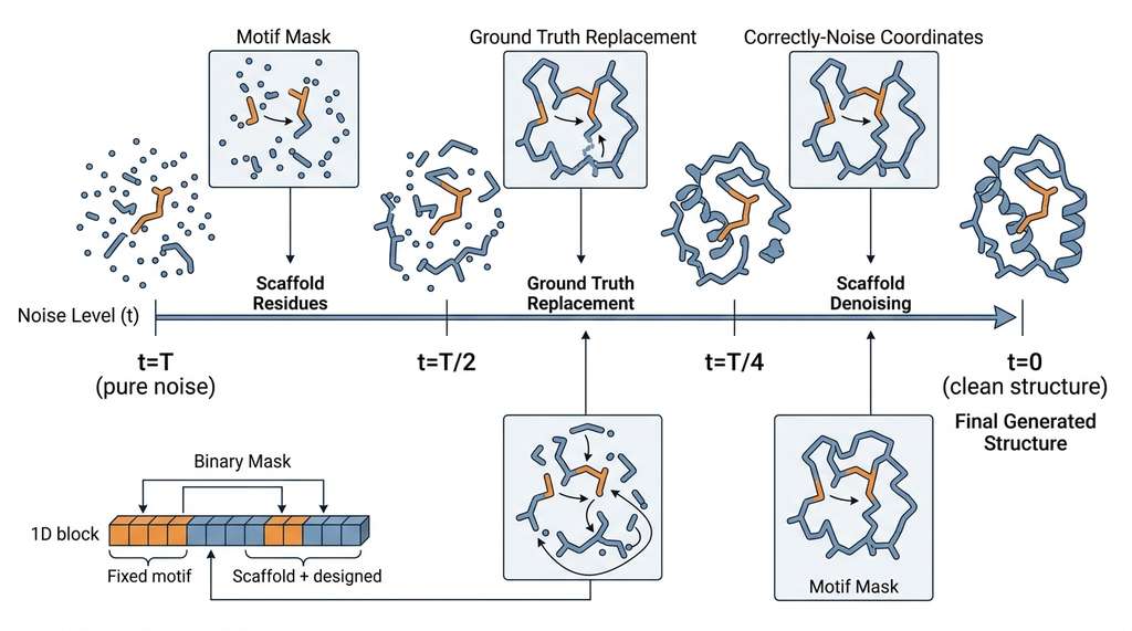
A particularly powerful form of conditional generation is inpainting: generating part of a structure while keeping another part fixed. For protein design, this enables motif scaffolding: given a functional motif (a binding site, a catalytic triad, an epitope), generate a complete protein backbone that positions the motif correctly and provides structural stability.
During the reverse diffusion process, each denoising step replaces values at fixed positions with the ground-truth motif noised to the current level. Scaffold regions generate freely while remaining structurally consistent with the motif. Figure 34.4.1 illustrates diffusion inpainting for motif scaffolding.
@torch.no_grad()
def inpainting_sample(model, motif_positions: torch.Tensor,
                      motif_mask: torch.Tensor, shape: tuple,
                      T: int, alpha_bars: torch.Tensor,
                      alphas: torch.Tensor, betas: torch.Tensor,
                      device: torch.device):
    """Generate structures with fixed motif regions via inpainting.

    Args:
        model: trained noise predictor
        motif_positions: ground truth positions for motif residues (N, 3)
        motif_mask: boolean mask, True for motif residues (N,)
        shape: output shape (N, 3)
        T: number of diffusion steps
    """
    # Start from noise
    x = torch.randn(shape, device=device)

    for t_val in reversed(range(T)):
        t = torch.full((1,), t_val, device=device, dtype=torch.long)
        alpha_bar_t = alpha_bars[t_val]

        # Standard reverse step for scaffold regions
        noise_pred = model(x, t)
        alpha_t = alphas[t_val]
        beta_t = betas[t_val]

        x_denoised = (1 / torch.sqrt(alpha_t)) * (
            x - (beta_t / torch.sqrt(1 - alpha_bar_t)) * noise_pred
        )

        if t_val > 0:
            noise = torch.randn_like(x)
            x_denoised = x_denoised + torch.sqrt(beta_t) * noise

        # Inpainting: replace motif positions with correctly noised ground truth
        if t_val > 0:
            motif_noise = torch.randn_like(motif_positions)
            alpha_bar_prev = alpha_bars[t_val - 1]
            motif_noisy = (torch.sqrt(alpha_bar_prev) * motif_positions +
                          torch.sqrt(1 - alpha_bar_prev) * motif_noise)
        else:
            motif_noisy = motif_positions  # final step: use clean motif

        # Blend: motif positions from ground truth, scaffold from generation
        mask = motif_mask.unsqueeze(-1).expand_as(x)
        x = torch.where(mask, motif_noisy, x_denoised)

return xConsider designing a novel enzyme that positions a serine-histidine-aspartate catalytic triad (the active site geometry found in serine proteases) within a structurally stable protein. Using RFDiffusion's motif scaffolding mode, you specify the 3D coordinates of the three catalytic residues as fixed constraints. The model generates thousands of diverse backbone scaffolds, each positioning the triad with sub-angstrom accuracy relative to the target geometry in reported experiments (Watson et al., 2023). ProteinMPNN then designs amino acid sequences for each scaffold, and AlphaFold2 (or, as of 2024, AlphaFold3, which handles ligands and nucleic acids natively) filters for designs whose predicted structures match the generated backbone. This pipeline has produced experimentally validated enzymes with catalytic activity, demonstrating that equivariant diffusion can design functional proteins from scratch. The catalytic triad specification requires 36 numbers (4 backbone atoms times 3 coordinates for each of the three catalytic residues); the model fills in the remaining 200+ residues.
3. REINFORCE for Non-Differentiable Rewards
Both classifier-free guidance and inpainting rely on information available during training: property labels or known structural motifs. Yet many of the properties that matter most for discovery can only be evaluated after a molecule is fully generated.
Classifier-free guidance works when the target property can be encoded as a conditioning signal during training. But many discovery-relevant properties cannot: docking scores require running a physics-based simulation, synthetic accessibility scores involve graph-based heuristics, and experimental binding affinity is only available after wet-lab testing. For these non-differentiable reward functions, policy gradient methods from reinforcement learning provide the solution.
The REINFORCE algorithm (Williams, 1992) treats the generative model as a policy \(\pi_\theta(x)\) that produces molecular samples \(x\), and the property evaluator as a reward function \(R(x)\). The objective is to maximize the expected reward:
$$J(\theta) = \mathbb{E}_{x \sim \pi_\theta}[R(x)]$$The gradient of this objective is given by the log-derivative trick (rewriting the gradient of an expectation as an expectation of the score function weighted by the reward, so that we never need to differentiate through \(R\) itself):
$$\nabla_\theta J(\theta) = \mathbb{E}_{x \sim \pi_\theta}[R(x) \cdot \nabla_\theta \log \pi_\theta(x)]$$This gradient does not require differentiating through the reward function \(R(x)\); it only requires evaluating \(R(x)\) and computing the log-probability \(\log \pi_\theta(x)\) of the generated sample. For autoregressive molecular generators, \(\log \pi_\theta(x)\) is the sum of log-probabilities at each generation step. For diffusion models, it can be approximated via the probability flow ordinary differential equation (ODE), which recasts the stochastic diffusion process as a deterministic trajectory whose log-likelihood can be computed exactly (Section 34.2).
Checkpoint
So far: REINFORCE treats the generator as a policy and the property evaluator as a reward, then uses the log-derivative trick to compute gradients without differentiating through the reward function; the only ingredients needed are the reward value and the log-probability of each generated sample.
Common Misconception
Readers often assume that REINFORCE trains the generator to produce only high-reward molecules, replacing the original chemical knowledge with reward-chasing behavior. This is incorrect: REINFORCE adjusts the sampling probabilities so that high-reward regions are visited more frequently, but the pretrained model's chemical grammar remains the foundation. Without safeguards (Kullback-Leibler (KL) penalty, entropy bonus), the distribution can collapse to a narrow mode, but the mechanism is probability reweighting, not replacement of learned chemistry. The generator never "forgets" how to make valid molecules; it shifts which valid molecules it prefers.
import torch
import torch.nn.functional as F
from typing import Callable, List
from dataclasses import dataclass


@dataclass
class RewardConfig:
    """Configuration for multi-property reward function."""
    weights: dict          # property_name -> weight
    thresholds: dict       # property_name -> minimum acceptable value
    baseline_ema: float    # exponential moving average decay for baseline


class REINFORCETrainer:
    """REINFORCE optimizer for molecular generators with non-differentiable rewards.

    Fine-tunes a pretrained autoregressive molecular generator
    to maximize a multi-property reward function.
    """
    def __init__(self, generator: torch.nn.Module,
                 reward_fns: dict,  # name -> callable(smiles) -> float
                 config: RewardConfig,
                 lr: float = 1e-5):
        self.generator = generator
        self.reward_fns = reward_fns
        self.config = config
        self.optimizer = torch.optim.Adam(generator.parameters(), lr=lr)
        self.baseline = 0.0  # running baseline for variance reduction

    def compute_reward(self, smiles_list: List[str]) -> torch.Tensor:
        """Compute multi-property reward for a batch of molecules."""
        rewards = torch.zeros(len(smiles_list))
        property_values = {}

        for name, fn in self.reward_fns.items():
            values = torch.tensor([fn(s) for s in smiles_list])
            property_values[name] = values

            # Apply threshold: zero reward if below minimum
            threshold = self.config.thresholds.get(name, float('-inf'))
            mask = values >= threshold

            # Weighted contribution
            weight = self.config.weights.get(name, 1.0)
            rewards += weight * values * mask.float()

        return rewards, property_values

    def train_step(self, batch_size: int = 64) -> dict:
        """One REINFORCE training step."""
        self.generator.train()

        # Generate molecules and collect log-probabilities
        samples, log_probs = self.generator.sample_with_log_prob(batch_size)

        # Decode to SMILES (generator-specific)
        smiles_list = self.generator.decode_to_smiles(samples)

        # Compute rewards (non-differentiable)
        rewards, properties = self.compute_reward(smiles_list)
        rewards = rewards.to(log_probs.device)

        # Update baseline (variance reduction): subtracting a near-mean
        # value from each reward centers the advantages around zero,
        # which sharply reduces gradient variance without introducing bias.
        self.baseline = (self.config.baseline_ema * self.baseline +
                        (1 - self.config.baseline_ema) * rewards.mean().item())

        # REINFORCE gradient: (R - baseline) * grad log pi
        advantage = rewards - self.baseline
        loss = -(advantage * log_probs).mean()

        # Optional: add entropy bonus to prevent mode collapse
        entropy = -(torch.exp(log_probs) * log_probs).mean()
        loss = loss - 0.01 * entropy

        self.optimizer.zero_grad()
        loss.backward()

        # Gradient clipping for stability
        torch.nn.utils.clip_grad_norm_(self.generator.parameters(), 1.0)
        self.optimizer.step()

        return {
            'loss': loss.item(),
            'mean_reward': rewards.mean().item(),
            'baseline': self.baseline,
            'entropy': entropy.item(),
            'valid_frac': sum(1 for s in smiles_list if s is not None) / len(smiles_list),
            'properties': {k: v.mean().item() for k, v in properties.items()}
}compute_reward applies per-property thresholds and weights, while the training loop uses the advantage (reward minus running baseline) to upweight high-scoring molecules.Step-Through: One REINFORCE Update
Trace through a single training step with a batch of 4 molecules, using QED (drug-likeness, range 0 to 1) as the reward. Suppose the generator samples four Simplified Molecular Input Line Entry System (SMILES) strings with log-probabilities and QED scores:
Molecule A: log p = −12.3, QED = 0.82
Molecule B: log p = −15.1, QED = 0.41
Molecule C: log p = −11.7, QED = 0.73
Molecule D: log p = −14.0, QED = 0.55
Step 1: Compute mean reward. baseline = (0.82 + 0.41 + 0.73 + 0.55) / 4 = 0.6275.
Step 2: Compute advantages. A: 0.82 − 0.6275 = +0.1925, B: 0.41 − 0.6275 = −0.2175, C: 0.73 − 0.6275 = +0.1025, D: 0.55 − 0.6275 = −0.0775.
Step 3: Compute loss contributions. Each term is −advantage × log p: A: −(+0.1925)(−12.3) = +2.368, B: −(−0.2175)(−15.1) = −3.284, C: −(+0.1025)(−11.7) = +1.199, D: −(−0.0775)(−14.0) = −1.085. Mean loss = (2.368 − 3.284 + 1.199 − 1.085) / 4 = −0.201.
Step 4: Interpret. The negative loss means the gradient update will increase the probability of molecules A and C (above-baseline QED) and decrease the probability of B and D (below-baseline QED). The magnitude of each molecule's contribution is proportional to both its advantage and its log-probability, so high-reward molecules that already have high probability get the largest positive push.
REINFORCE optimizes whatever reward function you give it, including the artifacts and biases of that function. If your docking score predictor has systematic errors for certain scaffolds, REINFORCE will find and exploit them. This is Goodhart's law applied to molecular design: "when a measure becomes a target, it ceases to be a good measure." Three defenses help. First, use multiple orthogonal reward components (docking score AND synthetic accessibility AND drug-likeness) so exploiting one requires satisfying the others. Second, include a KL penalty against the pretrained model to prevent the fine-tuned model from drifting too far from the space of valid molecules. Third, validate top candidates with independent tools: if your reward uses a fast docking proxy, re-score the top 100 molecules with a more expensive physics-based method. We implement all three safeguards in the recipe of Section 34.5.
4. Evaluation Metrics for Molecular Generators
How do you know if your molecular generator is any good? The evaluation landscape for generative models in chemistry and biology has matured into a set of standard metrics, organized into four categories.
Validity measures whether generated molecules satisfy basic chemical rules: correct valences, no impossible bonds, parseable SMILES strings. For SMILES-based generators, validity rates in published benchmarks range from 30% (early variational autoencoders, or VAEs) to 99%+ (graph-based generators with action masking, where the model's output space is restricted at each step to only chemically valid bond additions), a roughly threefold improvement driven primarily by switching from string representations to graph representations that enforce valence rules by construction. For 3D structure generators, validity includes bond length and angle distributions matching reference data.
Uniqueness measures the fraction of non-duplicate molecules among valid outputs. A generator that produces the same molecule 1000 times has 100% validity but 0.1% uniqueness. Mode collapse, where the generator's output distribution concentrates on a small number of nearly identical samples, in generative adversarial networks (GANs) manifests as low uniqueness.
Novelty measures the fraction of generated molecules not present in the training set. A generator that memorizes and replays training data has 100% validity and uniqueness but 0% novelty. High novelty is essential for discovery.
Validity, uniqueness, and novelty each diagnose a distinct failure mode: broken chemistry, mode collapse, and memorization, respectively.
Distribution similarity measures how closely the generated distribution matches a reference distribution. The Frechet ChemNet Distance (FCD; Preuer et al., 2018) computes the Frechet distance (a measure of how far apart two multivariate Gaussian fits to the activation vectors are) between the activations of a pretrained ChemNet model (a neural network trained on molecular activity data to learn general-purpose chemical representations) on generated and reference molecules, analogous to the Frechet Inception Distance (FID) score for images. Lower FCD indicates more similar distributions.
Internal diversity measures how different the generated molecules are from one another, complementing the four categories above. A generator may achieve high validity, uniqueness, and novelty yet still produce molecules clustered around a single scaffold. Internal diversity, computed as the average pairwise Tanimoto distance between molecular fingerprints, detects this clustering: values near 1.0 indicate highly diverse outputs, while values near 0.0 indicate near-identical structures differing only in minor substituents.
from rdkit import Chem
from rdkit.Chem import Descriptors, QED, AllChem
from collections import Counter
import numpy as np
from typing import List, Dict


class MolecularGeneratorEvaluator:
    """Evaluate molecular generators on standard metrics.

    Computes validity, uniqueness, novelty, property distributions,
    and internal diversity for a set of generated SMILES strings.
    """
    def __init__(self, training_smiles: set):
        self.training_smiles = training_smiles

    def evaluate(self, generated_smiles: List[str]) -> Dict[str, float]:
        """Compute all standard evaluation metrics."""
        n_total = len(generated_smiles)

        # Parse molecules, filtering invalid SMILES
        valid_mols = []
        valid_smiles = []
        for smi in generated_smiles:
            mol = Chem.MolFromSmiles(smi)
            if mol is not None:
                # Canonicalize for uniqueness checking
                canon = Chem.MolToSmiles(mol)
                valid_mols.append(mol)
                valid_smiles.append(canon)

        n_valid = len(valid_mols)
        validity = n_valid / n_total if n_total > 0 else 0.0

        # Uniqueness: fraction of distinct valid molecules
        unique_smiles = set(valid_smiles)
        uniqueness = len(unique_smiles) / n_valid if n_valid > 0 else 0.0

        # Novelty: fraction not in training set
        novel = unique_smiles - self.training_smiles
        novelty = len(novel) / len(unique_smiles) if unique_smiles else 0.0

        # Property distributions for valid molecules
        properties = self._compute_properties(valid_mols)

        # Internal diversity: average pairwise Tanimoto distance
        diversity = self._internal_diversity(valid_mols[:1000])  # cap for speed

        return {
            'validity': validity,
            'uniqueness': uniqueness,
            'novelty': novelty,
            'diversity': diversity,
            'n_valid': n_valid,
            'n_unique': len(unique_smiles),
            'n_novel': len(novel),
            **{f'mean_{k}': v for k, v in properties.items()}
        }

    def _compute_properties(self, mols: list) -> dict:
        """Compute molecular property statistics."""
        qed_scores = [QED.qed(m) for m in mols]
        mw = [Descriptors.MolWt(m) for m in mols]
        logp = [Descriptors.MolLogP(m) for m in mols]

        return {
            'QED': np.mean(qed_scores) if qed_scores else 0.0,
            'MW': np.mean(mw) if mw else 0.0,
            'LogP': np.mean(logp) if logp else 0.0,
        }

    def _internal_diversity(self, mols: list) -> float:
        """Average pairwise Tanimoto distance (higher = more diverse)."""
        if len(mols) < 2:
            return 0.0
        fps = [AllChem.GetMorganFingerprintAsBitVect(m, 2, 2048) for m in mols]
        from rdkit.DataStructs import BulkTanimotoSimilarity
        total_dist = 0.0
        n_pairs = 0
        for i in range(min(len(fps), 500)):  # cap pairwise comparisons
            sims = BulkTanimotoSimilarity(fps[i], fps[i+1:])
            total_dist += sum(1.0 - s for s in sims)
            n_pairs += len(sims)
        return total_dist / n_pairs if n_pairs > 0 else 0.0


# Usage example
evaluator = MolecularGeneratorEvaluator(training_smiles=set())
# results = evaluator.evaluate(generated_smiles_list)
# print(f"Validity: {results['validity']:.1%}")
# print(f"Uniqueness: {results['uniqueness']:.1%}")
# print(f"Novelty: {results['novelty']:.1%}")
# print(f"Diversity: {results['diversity']:.3f}")5. Benchmarks: MOSES, GuacaMol, and TDC
Standardized benchmarks enable fair comparison of molecular generators. Three dominate the field:
MOSES (Polykovskiy et al., 2020) provides a curated subset of ZINC, a freely available database of commercially available compounds for virtual screening, with standardized train/test splits and a comprehensive metric suite (validity, uniqueness, novelty, FCD, fragment similarity, scaffold similarity). It is the most widely used benchmark for unconditional molecular generation (as of 2024, MOSES is widely regarded as largely saturated for state-of-the-art models, with top methods achieving near-perfect scores on most metrics; the PMO benchmark described below and task-specific TDC leaderboards have become the preferred evaluation targets for goal-directed generation).
GuacaMol (Brown et al., 2019) focuses on goal-directed generation: given a target molecular property profile (e.g., high QED, LogP, the octanol-water partition coefficient measuring how readily a molecule crosses cell membranes, in range, specific scaffold), how well can the generator produce molecules matching the specification? This is more relevant for discovery than unconditional generation.
Therapeutic Data Commons (TDC) (Huang et al., 2021) provides real-world drug discovery tasks including absorption, distribution, metabolism, excretion, and toxicity (ADMET) prediction, drug-target interaction, and molecular generation benchmarks with clinically relevant endpoints. TDC is the closest to real discovery workflows and connects to the domain-specific applications in Chapter 49.
Checkpoint
So far: three standardized benchmarks partition the evaluation landscape: MOSES tests unconditional generation quality, GuacaMol tests goal-directed property targeting, and TDC connects to real-world drug discovery endpoints with clinically relevant tasks.
The evaluation code above implements metrics from scratch. The Therapeutic Data Commons provides standardized benchmark evaluation with a single function call:
from tdc import Evaluator

# Load the standard molecular generation evaluator
evaluator = Evaluator(name='Diversity')
diversity = evaluator(generated_smiles)

evaluator = Evaluator(name='Validity')
validity = evaluator(generated_smiles)

evaluator = Evaluator(name='FCD')
fcd_score = evaluator(generated_smiles, reference_smiles)

# Or run the full MOSES benchmark suite
from tdc import BenchmarkGroup
group = BenchmarkGroup(name='MolGen')
results = group.evaluate(generated_smiles)TDC handles all the canonical SMILES normalization, train/test split management, and metric computation that the from-scratch implementation requires, reducing the 80-line evaluator above to 5 lines. It also provides leaderboards for comparing against published methods.
Real-World Application: Drug Discovery at Insilico Medicine
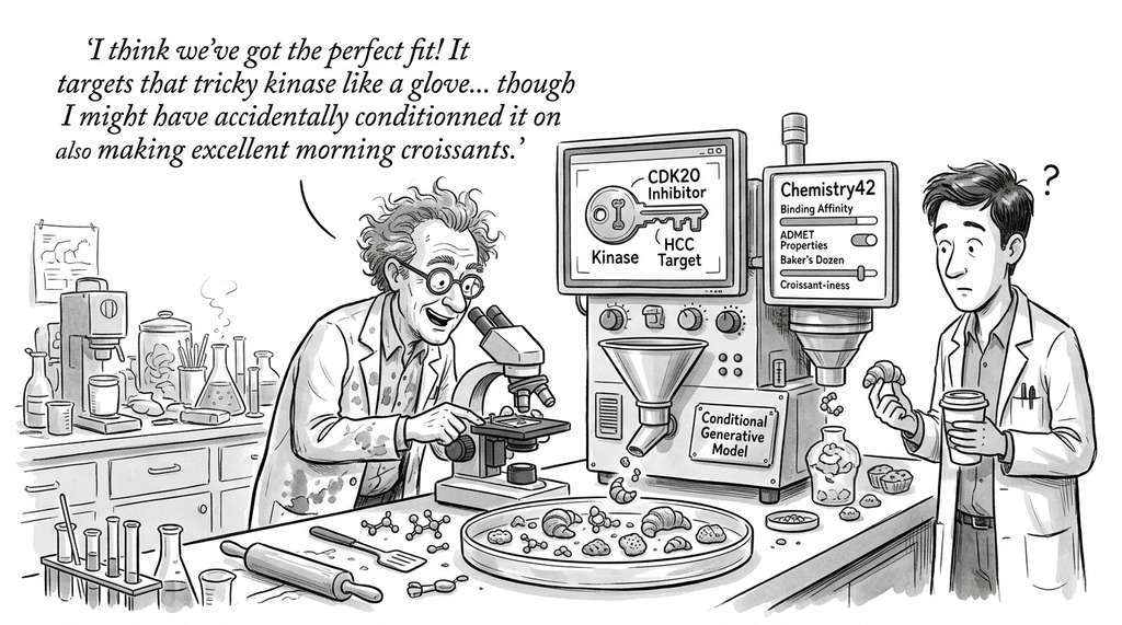
Insilico Medicine used a conditional generative model (Chemistry42) with REINFORCE-based optimization to design a novel inhibitor of CDK20, a kinase implicated in hepatocellular carcinoma. The generator was conditioned on binding affinity, ADMET properties, and synthetic accessibility simultaneously, producing candidates that satisfied all constraints. The top-ranked molecule entered preclinical testing within 18 months of generation, roughly one quarter of the typical timeline according to the company's published reports, suggesting that conditional molecular generation can compress the early stages of drug discovery from years to months.
The Generator That Rediscovered Aspirin
When researchers at BenevolentAI first benchmarked their conditional molecular generator on an anti-inflammatory reward function, the top-scoring output was acetylsalicylic acid: aspirin, patented in 1899. Far from being a failure, this became a useful sanity check. If a generator conditioned on a well-understood therapeutic property does not rediscover known drugs for that indication, something is wrong with the reward function. Several teams now include "known drug recovery rate" as a standard validation metric, turning a seemingly embarrassing result into a diagnostic tool.
The standard metrics (validity, uniqueness, novelty, FCD) evaluate the generator in isolation. But the real question for discovery is: do the generated molecules succeed in downstream experiments? The Practical Molecular Optimization (PMO) benchmark (Gao et al., 2022) took an early step by evaluating generators on their ability to optimize oracle functions within a budget of calls. More recently, DrugAgent (Li et al., 2024) introduces an LLM-powered multi-agent framework that integrates molecular generation with automated literature retrieval, ADMET filtering, and synthesis planning into a single closed-loop system, achieving state-of-the-art hit rates on multi-parameter optimization tasks from TDC. SynFlowNet (Cretu et al., 2024) constrains the generative process itself to only propose molecules constructible from purchasable building blocks via known reactions, so that every generated candidate is synthesizable by construction rather than by post-hoc filtering. The frontier is converging on evaluation protocols where computational generation feeds directly into robotic synthesis and assay, connecting to the self-driving laboratory paradigm of Chapter 55.
6. Putting It Together: The Conditional Generation Pipeline
A complete conditional generation pipeline for molecular discovery combines the components from this section into a coherent workflow. Figure 34.4.2 illustrates the five stages and the feedback loop that connects evaluation back to conditioning.
Stage 1: Pretrain. Train an unconditional or weakly conditional generative model on a large molecular dataset (ZINC, ChEMBL, a curated database of bioactive compounds with measured activity against biological targets, PubChem). This gives the model broad chemical knowledge: valid bond patterns, common functional groups, realistic size distributions.
Stage 2: Condition. Add conditioning signals via classifier-free guidance (differentiable properties) or prepare for REINFORCE fine-tuning (non-differentiable properties). For structure-based design, condition on the target protein pocket geometry.
Stage 3: Generate and filter. Generate a large pool of candidates (10,000+), filter by validity and basic property thresholds, and deduplicate.
Stage 4: Evaluate. Score filtered candidates with the full property prediction pipeline (docking, ADMET, synthesizability). Compute the standard metrics to verify the generator is working correctly.
Stage 5: Iterate. Feed top-scoring candidates back as conditioning signals or training data for the next round. This iterative refinement typically converges toward the target property region while maintaining diversity.
The next section implements this complete pipeline.
Try It: Evaluate a SMILES Generator from Scratch
Build a minimal molecular generation evaluation pipeline using only RDKit and NumPy.
(1) Install RDKit: pip install rdkit-pypi numpy.
(2) Create a baseline "generator" by randomly sampling 1,000 SMILES from the ZINC250K
dataset CSV (available from the MOSES GitHub repository); treat these as your "generated"
molecules and hold out 500 as a reference training set.
(3) Implement the four core metrics from this section: parse each SMILES with
Chem.MolFromSmiles() to compute validity, canonicalize with
Chem.MolToSmiles() and count unique strings for uniqueness, subtract the
training set for novelty, and compute pairwise Tanimoto distances on Morgan fingerprints (circular substructure fingerprints that encode the presence of molecular neighborhoods within a given bond radius as a fixed-length bit vector)
for internal diversity.
(4) Deliberately degrade your "generator" to observe metric trade-offs: duplicate each
molecule 5 times (watch uniqueness drop), restrict to training-set molecules only (watch
novelty drop), and insert random character strings (watch validity drop).
(5) Plot all four metrics across these degradation modes as a grouped bar chart with
matplotlib, reproducing the type of evaluation table found in MOSES benchmark papers.
Exercises
- (Conceptual) Explain why the guidance scale \(w\) in classifier-free guidance can be interpreted as controlling a temperature parameter on the conditional distribution. What happens to the entropy of the generated distribution as \(w \to \infty\)? How does this relate to the exploitation side of the exploration-exploitation trade-off from Chapter 1?
-
(Coding) Implement the
MolecularGeneratorEvaluatorfrom this section and evaluate two molecular generation strategies: (a) random sampling from a pretrained SMILES VAE, and (b) latent space optimization of the same VAE using a QED predictor as the objective. Compare validity, uniqueness, novelty, and mean QED for 1000 molecules from each strategy. Does the optimized generator sacrifice any metric to improve QED? - (Analysis) The REINFORCE estimator has notoriously high variance. Implement REINFORCE with and without the baseline variance reduction technique from this section. Generate 100 batches of 64 molecules each and plot the gradient variance (estimated as the variance of the per-sample gradient contributions) across batches. How much does the baseline reduce variance? Experiment with the baseline EMA decay parameter: what value gives the best variance-reward trade-off?
Exercise 34.4.1
Suppose you train a diffusion model with classifier-free guidance using \(p_{\text{uncond}} = 0.15\) and then sample with guidance scale \(w = 4.0\). Write out the guided noise prediction formula and compute the guided prediction \(\hat{\epsilon}\) when the unconditional model predicts \(\epsilon_{\text{uncond}} = 0.6\) and the conditional model predicts \(\epsilon_{\text{cond}} = 0.9\) (treating these as scalar values for simplicity). Then explain: if you increase \(w\) to 10.0, what happens to \(\hat{\epsilon}\), and why might this cause the generated molecule to violate chemical validity constraints?
Hint
Plug into \(\hat{\epsilon} = \epsilon_{\text{uncond}} + w \cdot (\epsilon_{\text{cond}} - \epsilon_{\text{uncond}})\). For \(w = 4\), the guided prediction is \(0.6 + 4.0 \times (0.9 - 0.6) = 1.8\). For \(w = 10\), repeat the same formula. Notice that the guided prediction can exceed the range the model was trained on. The denoiser learned to predict noise values within a certain distribution; extrapolating far beyond that range pushes the sample into regions the model never saw during training.
Lab: Guidance Scale Sweep on a Molecular Diffusion Model
Goal: Observe how classifier-free guidance scale affects the validity, diversity, and property targeting of generated molecules.
Tools: Python, RDKit (pip install rdkit-pypi), a pretrained SMILES-based VAE or autoregressive model (use the REINVENT or mol_gen package, or substitute any pretrained molecular generator you have access to), matplotlib.
Procedure (20 minutes): (1) Load or train a simple conditional molecular generator on ZINC250K, conditioning on LogP. (2) Generate 500 molecules at each guidance scale in {1.0, 2.0, 3.0, 5.0, 7.0, 10.0, 15.0}. (3) For each batch, compute validity (fraction parseable by RDKit), uniqueness (fraction of distinct canonical SMILES), internal diversity (mean pairwise Tanimoto distance on Morgan fingerprints), and mean LogP of valid molecules.
What to vary: The guidance scale \(w\).
What to observe: Plot all four metrics against \(w\). You should see mean LogP increase monotonically with \(w\), while validity and diversity decrease at high \(w\). Identify the "sweet spot" where LogP targeting is strong but validity remains above 90%. This is the exploration-exploitation trade-off in action.
What's Next
We have all the pieces: diffusion models for generation (Section 34.2), equivariant architectures for 3D structures (Section 34.3), and conditioning and evaluation mechanisms (this section). Section 34.5: Building a Molecular Generator assembles these into a complete, working pipeline: structure-based drug design with DiffSBDD-style diffusion, multi-property scoring with QED, synthetic accessibility, and a docking proxy, REINFORCE fine-tuning for target optimization, and integration with the Discovery Workbench.