48.2 Protein Structure and Design

1. Protein Structure Primer

A string of just 100 amino acids can fold into more possible shapes than there are atoms in the observable universe, yet cells reliably produce the same structure every time; understanding how sequence dictates fold is the key that unlocked both prediction and design. Structure is described at four levels:

• Primary: the amino acid sequence, a string over a 20-letter alphabet.
• Secondary: local structural motifs, primarily alpha-helices and beta-sheets, determined by backbone hydrogen bonding patterns.
• Tertiary: the full 3D arrangement of a single chain, specified by the coordinates of every atom (or, more compactly, by backbone torsion angles \(\phi\), \(\psi\), \(\omega\)).
• Quaternary: the arrangement of multiple chains in a complex.

The backbone geometry of each residue is described by three dihedral angles. The peptide bond angle \(\omega\) is nearly always 180 degrees (trans configuration), leaving two degrees of freedom per residue: \(\phi\) (rotation around the N-C\(_\alpha\) bond) and \(\psi\) (rotation around the C\(_\alpha\)-C bond). The Ramachandran plot, a two-dimensional map of sterically allowed \((\phi, \psi)\) combinations for each residue, shows which \((\phi, \psi)\) pairs are energetically favorable and which are forbidden by atomic clashes (see Section 33.3 for geometric constraints in molecular representations).

2. AlphaFold2: The Prediction Revolution

Before AlphaFold2, determining a single protein structure could take a graduate student an entire PhD and hundreds of thousands of dollars in synchrotron time; without that structure, drug designers were working blind, unable to see the molecular surface they needed to target. The ability to predict structure from sequence alone changed the economics of structural biology overnight.

AlphaFold2 (AF2) predicts protein structures with accuracy matching X-ray crystallography (median Global Distance Test Total Score (GDT-TS) > 92 on CASP14 free-modeling targets), where CASP14 is the 14th round of the Critical Assessment of protein Structure Prediction, a biennial blind competition that benchmarks structure prediction methods against unpublished experimental structures . Its architecture has two key innovations:

2.1 The Evoformer

AF2 processes two representations simultaneously. The first is a multiple sequence alignment (MSA) representation (a table of evolutionarily related protein sequences aligned position by position, so that each column corresponds to the same structural site) of shape \((N_{\text{seq}}, L, c_m)\). The second is a pair representation of shape \((L, L, c_z)\), where \(L\) is the sequence length. The evoformer block updates both through alternating attention operations:

1. Row-wise MSA attention: each row of the MSA (a homologous sequence) attends to other positions within the same row, biased by the pair representation. This captures intra-sequence correlations.
2. Column-wise MSA attention: each column of the MSA (a position across homologs) attends to the same position in other sequences. This captures evolutionary covariation, the signal that two positions covary across evolution because they are in spatial contact.
3. Pair update via outer product mean: the MSA representation updates the pair representation through an outer product of column vectors, converting coevolutionary signal into pairwise distance information.
4. Triangle attention and updates: the pair representation refines itself through operations that enforce geometric consistency (if residues \(i\) and \(j\) are close, and \(j\) and \(k\) are close, this constrains the \(i\)-\(k\) distance).

The pair representation \(z_{ij}\) encodes the relationship between every pair of residues. After 48 evoformer blocks, this representation contains sufficient information to determine the 3D structure.

2.2 Structure Module

The structure module converts the pair and MSA representations into 3D coordinates using Invariant Point Attention (IPA; "invariant" here refers to the fact that the final output is invariant to global coordinate changes, even though the internal computation is equivariant), which operates on rigid-body frames \((R_i, \mathbf{t}_i) \in \text{SE}(3)\), where SE(3) is the special Euclidean group in three dimensions representing all possible rotations and translations of a rigid body , attached to each residue. IPA computes attention scores using both the embedding space and the 3D coordinate space, ensuring that the attention is equivariant to global rotations and translations:

where \(\mathbf{q}_i, \mathbf{k}_j\) are query and key vectors in embedding space, \(\mathbf{p}^{(h)}\) are learned 3D query/key points, \(R_i, \mathbf{t}_i\) are the current frame for residue \(i\), and \(b_{ij}\) is a bias from the pair representation. The structure module iterates 8 times, refining the frames from an initial identity-frame configuration to the predicted structure. In short: prediction collapses billions of years of folding physics into a single forward pass; design inverts that pass to write sequences nature never tried.

2.3 Using AlphaFold3

AlphaFold3 (AF3) extends prediction to biomolecular complexes: protein-protein, protein-ligand, protein-nucleic acid, and even post-translationally modified proteins. Its architecture replaces the structure module with a diffusion-based generator that denoises atom coordinates from Gaussian noise, conditioned on the evoformer output. This allows AF3 to handle arbitrary molecular entities (small molecules, ions, modified residues) without specialized structure modules for each. As of late 2024, open-source alternatives such as Chai-1 and Boltz-1 have emerged, offering comparable biomolecular complex prediction with fully open weights and training code, broadening access beyond the AlphaFold ecosystem.

from Bio.PDB import PDBParser, PDBIO
import subprocess
import json

def predict_structure_alphafold3(
    sequences: list[str],
    job_name: str = "af3_prediction",
    output_dir: str = "./af3_output",
) -> dict:
    """Predict protein complex structure using AlphaFold3.

    Accepts multiple sequences for complex prediction.
    Returns paths to predicted structures and confidence scores.

    Requires: AlphaFold3 installed with model weights.
    """
    # Prepare input JSON for AF3
    input_data = {
        "name": job_name,
        "modelSeeds": [42],
        "sequences": [
            {"proteinChain": {"sequence": seq, "count": 1}}
            for seq in sequences
        ],
    }

    input_path = f"{output_dir}/{job_name}_input.json"
    with open(input_path, "w") as f:
        json.dump(input_data, f)

    # Run AF3 prediction
    subprocess.run([
        "python", "-m", "alphafold3",
        f"--json_path={input_path}",
        f"--output_dir={output_dir}",
        "--model_dir=/data/af3_weights",
    ], check=True)

    # Parse results
    result_dir = f"{output_dir}/{job_name}"
    return {
        "structure": f"{result_dir}/ranked_0.cif",
        "confidence": _parse_af3_confidence(result_dir),
    }


def _parse_af3_confidence(result_dir: str) -> dict:
    """Parse AlphaFold3 confidence metrics.

    predicted Local Distance Difference Test (pLDDT): per-residue confidence (0-100, >90 is high confidence)
    PAE: predicted aligned error between residue pairs
    ipTM: interface predicted Template Modeling score (TM-score) for complex accuracy
    """
    with open(f"{result_dir}/confidence.json") as f:
        conf = json.load(f)
    return {
        "plddt_mean": sum(conf["plddt"]) / len(conf["plddt"]),
        "iptm": conf.get("iptm", None),
        "ptm": conf["ptm"],
    }

3. ESMFold: Fast Single-Sequence Prediction

ESMFold typically achieves near-AF2 accuracy on single-domain proteins (within 1-2 GDT points on CASP14 single-chain targets, though the gap widens for multi-domain and low-homology targets) without requiring multiple sequence alignments. Instead, it uses a protein language model (ESM-2, with up to 15 billion parameters) pretrained on millions of protein sequences via masked language modeling. The key insight: the internal representations of a large language model trained on evolutionary data implicitly encode the same coevolutionary information that AF2 extracts explicitly from MSAs.

As of 2024, EvolutionaryScale released ESM3, a multimodal generative model that jointly reasons over sequence, structure, and function, extending the ESM family beyond prediction into programmable protein design. ESMFold's practical advantage is speed. AF2 requires computing MSAs against sequence databases (minutes to hours per protein); ESMFold runs in under a second for typical proteins on a single GPU, a 100 to 1000x speedup that turns structure prediction from a batch job into a real-time filter. This makes ESMFold ideal for filtering large numbers of designed sequences (as we do in Section 48.5).

import torch
import esm

def predict_structure_esmfold(sequence: str) -> dict:
    """Predict protein structure using ESMFold.

    Returns the predicted structure as a PDB string and
    per-residue pLDDT confidence scores.

    ESMFold processes a single sequence (no MSA needed),
    making it 100-1000x faster than AlphaFold2 per prediction.
    """
    model = esm.pretrained.esmfold_v1()
    model = model.eval().cuda()

    # Optionally reduce memory usage for long sequences
    model.set_chunk_size(128)

    with torch.no_grad():
        output = model.infer_pdb(sequence)

    # Extract per-residue confidence scores
    with torch.no_grad():
        result = model.infer(sequence)
        plddt = result["plddt"].cpu().numpy().squeeze()

    return {
        "pdb_string": output,
        "plddt_scores": plddt,
        "mean_plddt": float(plddt.mean()),
    }


def batch_predict_esmfold(
    sequences: list[str],
    min_plddt: float = 70.0,
) -> list[dict]:
    """Predict structures for many sequences and filter by confidence.

    Used in design pipelines to rapidly assess whether designed
    sequences are predicted to fold into the intended structure.
    """
    model = esm.pretrained.esmfold_v1()
    model = model.eval().cuda()
    model.set_chunk_size(128)

    results = []
    for i, seq in enumerate(sequences):
        with torch.no_grad():
            output = model.infer(seq)
            plddt = output["plddt"].cpu().numpy().squeeze()
            mean_plddt = float(plddt.mean())

        if mean_plddt >= min_plddt:
            results.append({
                "sequence": seq,
                "index": i,
                "mean_plddt": mean_plddt,
                "pdb_string": model.output_to_pdb(output)[0],
            })

    return sorted(results, key=lambda x: x["mean_plddt"], reverse=True)

from Bio.PDB import PDBParser, Superimposer
import numpy as np

def compute_rmsd(pdb_file1: str, pdb_file2: str) -> float:
    """Compute backbone root-mean-square deviation (RMSD) between two structures."""
    parser = PDBParser(QUIET=True)
    s1 = parser.get_structure("s1", pdb_file1)
    s2 = parser.get_structure("s2", pdb_file2)

    atoms1 = [a for a in s1.get_atoms() if a.name in ("N", "CA", "C", "O")]
    atoms2 = [a for a in s2.get_atoms() if a.name in ("N", "CA", "C", "O")]

    sup = Superimposer()
    sup.set_atoms(atoms1, atoms2)
    return sup.rms  # RMSD in Angstroms

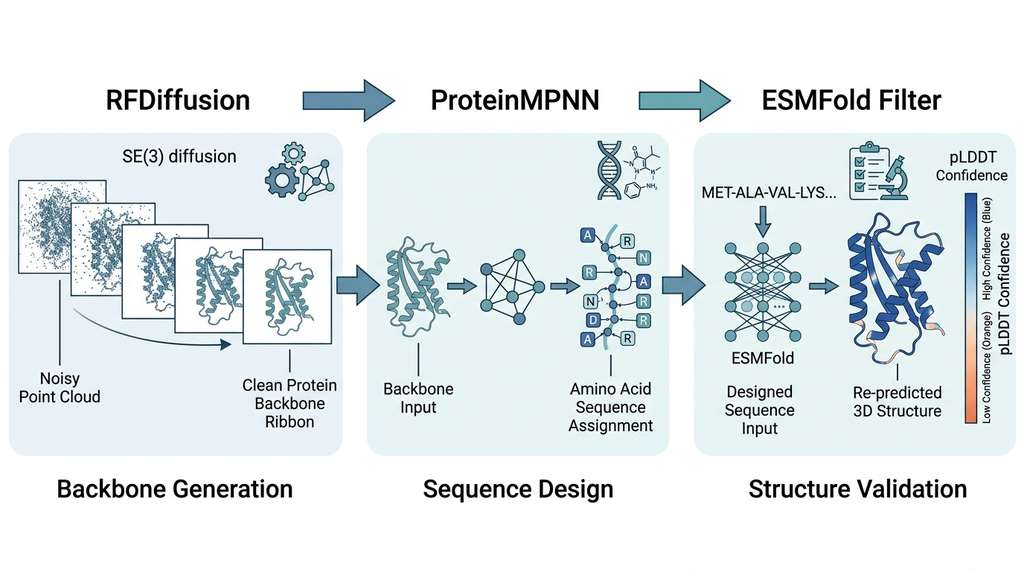
The three-stage protein design pipeline, from backbone generation through inverse folding to structure validation, is illustrated in Figure 48.2. The next two sections explain the generation and inverse-folding stages in detail; the figure provides a roadmap so you can see where each piece fits before diving in.

4. RFDiffusion: Generating Novel Protein Backbones

Predicting the structure of a known protein is powerful, but the greater prize is creating proteins that nature never built.

While AF2 and ESMFold predict the structure of natural proteins, RFDiffusion generates novel protein backbones that do not exist in nature. Built on the denoising diffusion framework from Chapter 34, RFDiffusion operates on the SE(3) manifold of rigid-body frames (as shown in Figure 48.2, Stage 1), diffusing protein backbone coordinates to noise and learning to reverse the process.

4.1 Diffusion on SE(3)

Each residue \(i\) is represented by a frame \(T_i = (R_i, \mathbf{t}_i) \in \text{SE}(3)\), where \(R_i \in \text{SO}(3)\) is a rotation matrix and \(\mathbf{t}_i \in \mathbb{R}^3\) is a translation. The forward diffusion process adds noise to both components:

For rotations, the noise is applied via the Lie algebra \(\mathfrak{so}(3)\), the tangent space of SO(3) at the identity that parameterizes infinitesimal rotations as 3D vectors :

where \(\exp(\cdot)\) is the exponential map from \(\mathfrak{so}(3)\) to SO(3). The reverse process uses RoseTTAFold as the denoising network, predicting clean frames from noisy frames at each diffusion timestep.

Mental Model

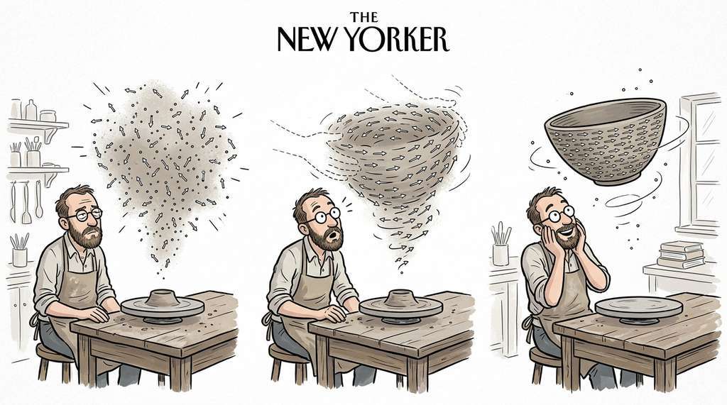
Think of SE(3) diffusion as sculpting from a fog of clay dust. Each residue starts as a grain of dust drifting in random position and orientation (pure noise). At each denoising step, the network nudges every grain toward a coherent shape, the way a potter's hands gradually compress loose clay into a recognizable bowl. The rotation component (SO(3)) controls the tilt of each grain; the translation component (\(\mathbb{R}^3\)) controls where it sits. Early steps establish the rough silhouette (helix here, sheet there), while later steps refine exact bond angles and inter-residue contacts. The critical difference from image diffusion: the "pixels" here are rigid bodies with orientation, so the noise schedule must respect curved geometry (the SO(3) manifold) rather than adding Gaussian noise in flat Euclidean space.

4.2 Design Modes

RFDiffusion supports several design modes, each specified by different conditioning:

• Unconditional generation: generate novel folds with no structural constraints. Specify only the desired length.
• Motif scaffolding: design a protein that places a functional motif (e.g., a binding epitope, where an epitope is the specific surface region recognized by an antibody or receptor) in a specified position within a novel scaffold . The motif residues are fixed; the surrounding structure is generated.
• Binder design: generate a protein that binds a specified target protein surface. The target structure is provided as context.
• Symmetric design: generate symmetric assemblies (dimers, trimers, icosahedral cages) with specified symmetry operations.

import subprocess
from pathlib import Path

def run_rfdiffusion(
    output_dir: str,
    contigs: str,
    num_designs: int = 100,
    target_pdb: str = None,
    hotspot_residues: list[str] = None,
    diffusion_steps: int = 50,
) -> list[str]:
    """Run RFDiffusion to generate protein backbone designs.

    Args:
        contigs: Residue specification string.
            "100" = unconditional, 100 residues
            "A1-50/0 70-100" = scaffold motif from residues 1-50
                of chain A with 70-100 new residues
        target_pdb: PDB file for binder design conditioning
        hotspot_residues: Target residues to design binders against
        diffusion_steps: Number of denoising steps (50 is standard)

    Returns: list of paths to generated PDB backbone files
    """
    cmd = [
        "python", "scripts/run_inference.py",
        f"inference.output_prefix={output_dir}/design",
        f"inference.num_designs={num_designs}",
        f"contigmap.contigs=[{contigs}]",
        f"diffuser.T={diffusion_steps}",
    ]

    if target_pdb is not None:
        cmd.append(f"inference.input_pdb={target_pdb}")

    if hotspot_residues is not None:
        hotspots = ",".join(hotspot_residues)
        cmd.append(f"ppi.hotspot_res=[{hotspots}]")

    subprocess.run(cmd, check=True, cwd="/path/to/RFdiffusion")

    # Collect generated backbone PDB files
    output_path = Path(output_dir)
    return sorted(str(p) for p in output_path.glob("design_*.pdb"))


# Example: unconditional generation of 100-residue proteins
backbones = run_rfdiffusion(
    output_dir="./designs/unconditional",
    contigs="100",
    num_designs=50,
)

# Example: binder design against a target protein
binder_backbones = run_rfdiffusion(
    output_dir="./designs/binders",
    contigs="A1-150/0 70-100",
    target_pdb="target.pdb",
    hotspot_residues=["A30", "A33", "A34"],
    num_designs=100,
)

5. ProteinMPNN: From Backbone to Sequence

RFDiffusion generates protein backbones (3D coordinates without amino acid identities). The inverse folding problem asks: which amino acid sequence will fold into this backbone? ProteinMPNN solves this using a message-passing neural network that takes backbone coordinates as input and outputs a probability distribution over amino acids at each position.

Inverse folding finds a sequence that spontaneously folds into a given backbone. Generative models like RFDiffusion produce backbones with no associated sequence, and a protein cannot be synthesized without one. ProteinMPNN encodes the backbone as a spatial graph and predicts, residue by residue, which amino acid best satisfies local geometry and chemistry. Use inverse folding whenever you have a target backbone from any source; use direct sequence optimization when you lack a backbone and want to search sequence space via a fitness function.

The model processes the protein as a \(k\)-nearest-neighbor graph (a graph where each residue is connected to the \(k\) residues closest to it in 3D space) in 3D space. Each node (residue) receives messages from its spatial neighbors, and the network autoregressively samples amino acids conditioned on the backbone geometry and previously sampled residues:

where \(\mathbf{s}\) is the sequence, \(\mathbf{X}\) are the backbone coordinates, and $s_{<i}$ denotes previously sampled residues. The autoregressive factorization allows diverse sampling: running the model multiple times with different random seeds produces different valid sequences for the same backbone.

import subprocess
import json

def run_proteinmpnn(
    pdb_path: str,
    output_dir: str,
    num_sequences: int = 8,
    temperature: float = 0.1,
    fixed_positions: dict = None,
) -> list[dict]:
    """Design sequences for a protein backbone using ProteinMPNN.

    Args:
        pdb_path: path to backbone PDB (from RFDiffusion or experiment)
        num_sequences: number of diverse sequences to generate
        temperature: sampling temperature (lower = more conservative)
        fixed_positions: dict mapping chain to list of fixed residue indices

    Returns: list of designed sequences with scores
    """
    cmd = [
        "python", "protein_mpnn_run.py",
        "--pdb_path", pdb_path,
        "--out_folder", output_dir,
        "--num_seq_per_target", str(num_sequences),
        "--sampling_temp", str(temperature),
        "--seed", "42",
        "--batch_size", "1",
    ]

    if fixed_positions is not None:
        # Write fixed positions JSON
        fixed_path = f"{output_dir}/fixed_positions.json"
        with open(fixed_path, "w") as f:
            json.dump(fixed_positions, f)
        cmd.extend(["--fixed_positions_jsonl", fixed_path])

    subprocess.run(cmd, check=True, cwd="/path/to/ProteinMPNN")

    # Parse output sequences
    results = []
    fasta_path = f"{output_dir}/seqs/{Path(pdb_path).stem}.fa"
    with open(fasta_path) as f:
        lines = f.readlines()
    for i in range(0, len(lines), 2):
        header = lines[i].strip()
        sequence = lines[i + 1].strip()
        # Parse score from header
        score = float(header.split("score=")[1].split(",")[0])
        results.append({
            "sequence": sequence,
            "score": score,
            "recovery": _compute_sequence_recovery(pdb_path, sequence),
        })

    return sorted(results, key=lambda x: x["score"])

5.1 LigandMPNN

LigandMPNN extends ProteinMPNN to design sequences in the context of bound ligands (small molecules, metal ions, nucleic acids). The network receives both backbone coordinates and ligand atom positions, designing sequences that form favorable interactions with the ligand. This is essential for enzyme design (where the active site must accommodate a substrate) and receptor design (where the binding pocket must complement a drug molecule).

In practice, LigandMPNN is invoked with the same command-line interface as ProteinMPNN, with an additional flag pointing to the ligand coordinates. You supply a PDB file containing both the protein backbone and the bound ligand (or metal ion), and LigandMPNN conditions its sequence predictions on the ligand atoms within a specified distance cutoff (typically 4 to 5 angstroms). The key difference from vanilla ProteinMPNN: residues near the ligand receive context about the ligand's chemistry, so the designed sequences are more likely to form productive contacts (hydrogen bonds, hydrophobic packing, metal coordination) with the bound molecule. Use LigandMPNN instead of ProteinMPNN whenever your design target includes a non-protein component that the designed sequence must accommodate.

6. FrameDiff and FoldFlow: Alternative Generative Approaches

Backbone generation and inverse folding form the two core stages of the design pipeline, and multiple algorithms compete on the generation side.

RFDiffusion is not the only approach to protein backbone generation. Two alternatives offer different trade-offs:

FrameDiff formulates backbone generation as diffusion on the product manifold \(\text{SE}(3)^L\), where each residue has an independent frame. The key difference from RFDiffusion: FrameDiff uses a simpler network architecture (a modified version of IPA from AlphaFold2) and trains on the full PDB without requiring the RoseTTAFold backbone. This makes it easier to retrain on custom datasets. The trade-off is generally lower designability (the fraction of generated backbones for which ProteinMPNN can find a sequence that ESMFold predicts will refold to the intended structure) on unconditional generation benchmarks, though the gap varies by target topology.

Flow Matching as an Alternative

FoldFlow replaces diffusion with continuous normalizing flows on SE(3), using Riemannian flow matching. Instead of learning a denoising process, FoldFlow learns a vector field that transports samples from a simple base distribution to the data distribution along geodesics (shortest paths on a curved manifold) on the SE(3) manifold :

where \(v_\theta\) is a learned vector field on SE(3). Flow matching avoids the need for reverse-process simulation and can be more sample-efficient than diffusion.

7. The Structure-to-Function Gap

Current protein design tools have a critical limitation: correct folding does not guarantee correct function. A designed enzyme might fold into the intended shape yet fail to catalyze the target reaction because the backbone representation does not capture subtle electronic or dynamic effects. Bridging this gap requires:

• Molecular dynamics simulations to assess conformational dynamics and binding thermodynamics (connecting to Chapter 43).
• Quantum chemistry calculations for active-site electronic structure.
• Experimental validation, which remains the ultimate arbiter. The fastest path from design to experiment is the self-driving laboratory (Chapter 55).

8. Discovery Workbench Integration

The Discovery Workbench gains a ProteinDesigner component that wraps the RFDiffusion, ProteinMPNN, and ESMFold pipeline (Figure 48.2) into a single interface. Users specify the design task (unconditional, motif scaffolding, or binder design), and the component orchestrates backbone generation, sequence design, structure validation, and ranking. All intermediate results are logged to the experiment registry for provenance tracking. Figure 48.2.1 illustrates Protein design pipeline from backbone generation to sequence validation.

from discovery_workbench import Designer, ExperimentRegistry

class ProteinDesigner(Designer):
    """Protein design pipeline for the Discovery Workbench."""

    def design_binder(
        self,
        target_pdb: str,
        hotspot_residues: list[str],
        num_backbones: int = 100,
        seqs_per_backbone: int = 8,
        min_plddt: float = 75.0,
    ) -> list[dict]:
        """Design proteins that bind a specified target.

        Pipeline: RFDiffusion -> ProteinMPNN -> ESMFold filtering
        """
        # Step 1: Generate backbones
        backbones = run_rfdiffusion(
            output_dir=self.work_dir / "backbones",
            contigs="A1-150/0 70-100",
            target_pdb=target_pdb,
            hotspot_residues=hotspot_residues,
            num_designs=num_backbones,
        )
        self.registry.log("backbone_generation", {"n": len(backbones)})

        # Step 2: Design sequences for each backbone
        all_designs = []
        for bb_path in backbones:
            seqs = run_proteinmpnn(
                pdb_path=bb_path,
                output_dir=self.work_dir / "sequences",
                num_sequences=seqs_per_backbone,
            )
            for seq_info in seqs:
                seq_info["backbone"] = bb_path
            all_designs.extend(seqs)
        self.registry.log("sequence_design", {"n": len(all_designs)})

        # Step 3: Filter by ESMFold confidence
        validated = batch_predict_esmfold(
            [d["sequence"] for d in all_designs],
            min_plddt=min_plddt,
        )
        self.registry.log("esmfold_filter", {
            "input": len(all_designs),
            "passed": len(validated),
        })

        return validated