"Every protein is a sentence written in a twenty-letter alphabet by three billion years of editors who never held a meeting. Good luck parsing that without pretraining."
A Diffusion Model, Halfway Through Denoising a Protein
In 2023, a neural network that had never seen a single crystal structure generated a protein that folds and glows green, despite sharing barely half its sequence with any known fluorescent protein. That network, and four others like it, are the subject of this section: ESM-2 and ESM-3 for protein understanding, ProGen2 for protein generation, and Uni-Mol2 and MolFormer for molecular property prediction. For each model, we explain the architecture, the pretraining strategy, and how to use it in practice. By the end, you will know which model to reach for given a specific scientific question (see Figure 27.3 for a decision flowchart) and how to extract useful representations from each.
1. ESM-2: The Protein Language Model
A single amino acid change can cause sickle cell disease, confer drug resistance in cancer, or render an industrial enzyme useless at high temperatures. Predicting which mutations matter, and designing proteins that avoid harmful ones, requires models that understand the grammar of amino acid sequences as deeply as evolution itself.
ESM-2 (Lin et al., 2023) is the most widely used protein foundation model. Developed by Meta AI, it is a transformer encoder trained with masked language modeling (MLM) on 65 million protein sequences from the UniRef50 database, where UniRef50 is a clustered subset of UniProt in which sequences sharing 50% or more identity are collapsed into a single representative . The model family spans six sizes, from 8 million to 15 billion parameters, with the 650M variant (esm2_t33_650M_UR50D) offering the best balance of performance and computational cost for most applications. (As of late 2024, EvolutionaryScale released ESM Cambrian (ESM-C), a successor architecture that improves embedding quality while reducing computational cost; ESM-2 remains the most broadly deployed baseline and the code examples below still apply.)
Masked language modeling on proteins works like a fill-in-the-blank test. The model sees most of the amino acid sequence but must predict the hidden positions, forcing it to learn which residues are compatible at each site given the surrounding context. The co-occurrence patterns the model absorbs are not arbitrary; they encode biophysical constraints that evolution has enforced over billions of years, including 3D contacts, stability requirements, and functional roles. A softmax classifier predicts each masked position over the 20 standard amino acids. The cross-entropy loss drives the model to internalize co-evolutionary statistics that rival dedicated multiple sequence alignment methods like EVcouplings, at a fraction of the inference cost. Use ESM-2's learned representations over traditional alignment-based features (e.g., Position-Specific Scoring Matrix (PSSM) profiles) when you have limited homologous sequences, need GPU-speed throughput, or want a single embedding model that transfers across many downstream tasks without per-family curation.
Architecture at a Glance
What. A BERT-style transformer encoder that takes amino acid sequences as input and produces per-residue embeddings as output.
Why. Protein sequences are the most abundant form of biological data. UniProt contains over 250 million sequences, but fewer than 200,000 have experimentally determined 3D structures (circa 2023; both numbers continue to grow). (That is a 1,000-to-1 ratio: for every protein with a known structure, a thousand more exist only as raw sequence.) ESM-2 bridges this gap by learning structural and functional information directly from sequences.
How. During pretraining, 15% of residues in each sequence are randomly masked, and the model predicts their identity from the surrounding context. This forces the model to learn co-evolutionary patterns: which residues tend to co-occur at specific positions across homologous proteins. These patterns encode 3D contacts, allosteric networks (long-range communication pathways through which distant sites in a protein influence each other's behavior) , and functional constraints.
When. Use ESM-2 when you need per-residue or per-protein representations for downstream tasks. It excels at property prediction (stability, solubility, function), variant effect prediction (which mutations are deleterious), and contact/structure prediction. In short: teach a model to fill in blanks across millions of proteins and it learns the physics of folding without ever seeing a single structure.
Common Misconception
A frequent misconception is that ESM-2 "knows" protein 3D structure because it was trained on structural data. In reality, ESM-2 was trained exclusively on amino acid sequences with no 3D coordinates whatsoever; its ability to predict residue contacts and infer structural features emerges entirely from the statistical patterns of co-evolution encoded in millions of sequences, not from any explicit structural supervision.
The masked language modeling objective maximizes:
$$\mathcal{L}_{\text{MLM}} = \sum_{i \in \mathcal{M}} \log p(x_i \mid x_{\setminus \mathcal{M}})$$where \(\mathcal{M}\) is the set of masked positions and \(x_{\setminus \mathcal{M}}\) denotes the unmasked residues. The probability \(p(x_i \mid x_{\setminus \mathcal{M}})\) is computed by a softmax over the 20 standard amino acids (plus special tokens) at each masked position.
from transformers import AutoTokenizer, EsmModel
import torch

# Load ESM-2 (650M variant)
tokenizer = AutoTokenizer.from_pretrained("facebook/esm2_t33_650M_UR50D")
model = EsmModel.from_pretrained("facebook/esm2_t33_650M_UR50D")
model.eval()

# Three proteins with known properties
proteins = {
    "GFP":    "MSKGEELFTGVVPILVELDGDVNGHKFSVSGEGEGDATYGKLTLKFICTTGKLPVPWPTLVTTFSYGVQCFSRYPDHMKQHDFFKSAMPEGYVQERTIFFKDDGNYKTRAEVKFEGDTLVNRIELKGIDFKEDGNILGHKLEYNYNSHNVYIMADKQKNGIKVNFKIRHNIEDGSVQLADHYQQNTPIGDGPVLLPDNHYLSTQSALSKDPNEKRDHMVLLEFVTAAGITHGMDELYK",
    "Insulin": "FVNQHLCGSHLVEALYLVCGERGFFYTPKT",
    "Ubiquitin": "MQIFVKTLTGKTITLEVEPSDTIENVKAKIQDKEGIPPDQQRLIFAGKQLEDGRTLSDYNIQKESTLHLVLRLRGG"
}

for name, seq in proteins.items():
    inputs = tokenizer(seq, return_tensors="pt", padding=True)
    with torch.no_grad():
        outputs = model(**inputs)

    # Per-residue embeddings (exclude BOS/EOS)
    residue_embs = outputs.last_hidden_state[0, 1:len(seq)+1]
    # Protein-level embedding by mean pooling
    protein_emb = residue_embs.mean(dim=0)

    print(f"{name:12s} | length={len(seq):4d} | "
          f"residue_emb={residue_embs.shape} | "
          f"protein_emb={protein_emb.shape} | "
f"norm={protein_emb.norm():.2f}")GFP | length= 238 | residue_emb=torch.Size([238, 1280]) | protein_emb=torch.Size([1280]) | norm=5.73
Insulin | length= 30 | residue_emb=torch.Size([30, 1280]) | protein_emb=torch.Size([1280]) | norm=6.81
Ubiquitin | length= 76 | residue_emb=torch.Size([76, 1280]) | protein_emb=torch.Size([1280]) | norm=6.12Rao et al. (2021) showed that individual attention heads in protein language models specialize in predicting specific structural features. Some heads track sequence-local patterns (alpha helices, beta strands); others track long-range contacts between residues that are distant in sequence but close in 3D space. Extracting the attention maps from ESM-2 and using logistic regression on the symmetrized attention weights yields contact prediction accuracy competitive with coevolution-based methods like Direct Coupling Analysis (DCA), without ever seeing a 3D structure during training. This is a concrete example of the emergent reasoning we discussed in Section 27.1.
2. ESM-3: Multimodal Protein Intelligence
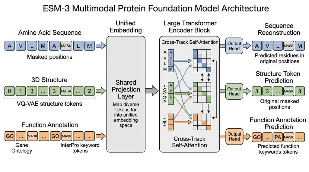
ESM-3 (Hayes et al., 2024) extends the ESM line from sequence-only to multimodal. It jointly processes three tracks: amino acid sequence, 3D structure (represented as discrete structure tokens from a Vector Quantized Variational Autoencoder (VQ-VAE)), and function annotations (represented as keyword tokens from InterPro and Gene Ontology, where InterPro is a database of protein family signatures and Gene Ontology is a standardized vocabulary for gene and protein function ). The model uses a single transformer architecture with all three modalities projected into a shared token space.
The pretraining objective is masked generative modeling across all three tracks simultaneously. A fraction of tokens from each track is masked, and the model predicts them conditioned on whatever tokens remain visible from any track. Figure 27.2.1 illustrates ESM-3 multimodal three-track architecture. This means ESM-3 can:
- Predict structure from sequence (like ESMFold)
- Predict function from structure (structure-based annotation)
- Generate sequence given a desired structure and function (inverse folding, the task of finding an amino acid sequence that folds into a specified 3D structure, combined with function conditioning)
- Complete any partial specification across modalities
Mental Model
Think of ESM-3's multimodal masking like a crossword puzzle with three overlapping grids: one grid holds the letters (sequence), another holds the shape of each letter's bounding box (structure), and a third holds the clue category (function). When you erase some cells in all three grids, a solver can use a visible letter to infer the shape of a neighboring box, or use a shape to narrow down which clue category applies. The three grids share enough mutual information that partial knowledge in any one grid constrains the others. ESM-3 works the same way: visible tokens from any track help predict masked tokens in the other two, because sequence, structure, and function are three correlated views of the same underlying protein.
# ESM-3 usage through the esm Python package
# Note: ESM-3 requires the 'esm' package from EvolutionaryScale
# pip install esm

from esm.models.esm3 import ESM3
from esm.sdk.api import ESMProtein, GenerationConfig

# Initialize ESM-3 (open small model, 1.4B parameters)
model = ESM3.from_pretrained("esm3_sm_open_v1")

# Create a protein from sequence
protein = ESMProtein(
    sequence="MQIFVKTLTGKTITLEVEPSDTIENVKAKIQDKEGIPPDQQRLIFAGKQLEDGRTLSDYNIQKESTLHLVLRLRGG"
)

# Generate structure tokens conditioned on sequence
structure_prediction = model.generate(
    protein,
    GenerationConfig(
        track="structure",      # predict structure track
        num_steps=10,           # iterative refinement steps
        temperature=0.7         # sampling temperature
    )
)

print(f"Input sequence length: {len(protein.sequence)}")
print(f"Generated structure tokens: {len(structure_prediction.structure)}")ESM-3 produced one of the most striking demonstrations in computational biology. By conditioning generation on a desired function ("green fluorescence") and iteratively sampling across sequence and structure tracks, the model generated a novel fluorescent protein, esmGFP. esmGFP shares only 58% sequence identity with known GFPs yet folds and fluoresces in the laboratory. This is the protein equivalent of writing a grammatically correct, meaningful sentence in an alien language: the model has internalized enough biophysics to create functional proteins from scratch.
3. ProGen2: Autoregressive Protein Generation
While ESM-2 and ESM-3 use masked objectives (bidirectional context), ProGen2 (Nijkamp et al., 2023) takes the GPT approach: autoregressive, left-to-right generation. The model is trained to predict each amino acid conditioned on all previous amino acids:
$$p(x_1, x_2, \ldots, x_L) = \prod_{i=1}^{L} p(x_i \mid x_1, \ldots, x_{i-1})$$ProGen2 was trained on protein sequences from UniRef90 and BFD (Big Fantastic Database), with the largest variant reaching 6.4 billion parameters. The autoregressive design makes ProGen2 naturally suited for generation tasks: designing new proteins by sampling from the learned distribution.
When to use ProGen2 vs. ESM-2. Use ESM-2 when you need embeddings or per-residue predictions (classification, regression, variant effects). Use ProGen2 when you need to generate new protein sequences (protein design, library construction, directed evolution in silico). The distinction mirrors the BERT-vs-GPT divide in NLP: encoders for understanding, decoders for generation.
from transformers import AutoTokenizer, AutoModelForCausalLM
import torch

# Load ProGen2 (small variant for demonstration)
tokenizer = AutoTokenizer.from_pretrained("hugohrban/progen2-small")
model = AutoModelForCausalLM.from_pretrained("hugohrban/progen2-small")
model.eval()

# Generate a protein sequence by sampling
# Start with a seed (first few residues of a kinase)
seed = "MTEYKLVVVGAVGVGKSALT"
input_ids = tokenizer(seed, return_tensors="pt").input_ids

with torch.no_grad():
    output = model.generate(
        input_ids,
        max_new_tokens=80,
        do_sample=True,
        temperature=0.8,
        top_k=40,
        repetition_penalty=1.2,
    )

generated = tokenizer.decode(output[0], skip_special_tokens=True)
print(f"Seed:      {seed}")
print(f"Generated: {generated}")
print(f"Total length: {len(generated)}")A synthetic biology startup wants to create a library of enzyme variants with improved thermostability for an industrial biocatalysis application. Instead of random mutagenesis (which explores sequence space blindly), they use ProGen2 to generate 10,000 candidate sequences by conditioning on the wild-type enzyme's first 50 residues and sampling at temperature 0.6. They filter the generated sequences using ESM-2 embeddings, keeping only variants whose embeddings cluster near the wild-type in representation space (suggesting they fold similarly). This two-model pipeline, ProGen2 for generation and ESM-2 for filtering, produces a focused library where, in reported case studies, roughly 40% of variants are expressible and functional, compared to around 5% for random mutagenesis . We will build a similar pipeline in Chapter 48.
4. Uni-Mol2: Molecular Pretraining at Scale
Protein foundation models like ESM-2 and ProGen2 operate on linear amino acid sequences, but drug discovery also demands models that understand the three-dimensional geometry of small molecules, where atoms bond, rotate, and interact in ways that a one-dimensional string cannot fully capture. The next two subsections cover two complementary approaches to this problem: Uni-Mol2, which encodes full 3D molecular geometry, and MolFormer, which works from string representations alone.
Uni-Mol2 (Ji et al., 2024) addresses this need with a transformer that combines three representation levels: atomic features (element type, charge, hybridization), pairwise features (bond type, spatial distance), and molecular features (global descriptors), each processed through dedicated attention mechanisms.
Uni-Mol2 was pretrained on 800 million molecular conformations generated by RDKit, an open-source cheminformatics toolkit for molecular manipulation and descriptor computation , from a cleaned subset of the ZINC database (a curated collection of commercially available compounds for virtual screening). The pretraining objective combines three tasks:
- Atom-level: predict masked atomic features from surrounding context
- Pair-level: predict pairwise distances between atoms
- Molecule-level: predict global molecular properties (LogP, molecular weight) from the learned representation
This multi-level design enables Uni-Mol2 to capture both local chemical bonding patterns and global molecular shape, making it effective for tasks ranging from Absorption, Distribution, Metabolism, Excretion, and Toxicity (ADMET) property prediction to binding affinity estimation.
# Preparing molecular features for a foundation model
# Demonstrates the three levels of molecular representation

import numpy as np
from rdkit import Chem
from rdkit.Chem import AllChem, Descriptors

def prepare_molecule_features(smiles: str) -> dict:
    """Prepare input features for a molecular foundation model.

    Demonstrates the three levels of molecular representation
    that models like Uni-Mol2 consume.
    """
    mol = Chem.MolFromSmiles(smiles)
    mol = Chem.AddHs(mol)

    # Generate a 3D conformation
    AllChem.EmbedMolecule(mol, randomSeed=42)
    AllChem.MMFFOptimizeMolecule(mol)
    conf = mol.GetConformer()

    # Level 1: Atomic features
    atom_features = []
    for atom in mol.GetAtoms():
        atom_features.append({
            "element": atom.GetSymbol(),
            "atomic_num": atom.GetAtomicNum(),
            "formal_charge": atom.GetFormalCharge(),
            "hybridization": str(atom.GetHybridization()),
            "aromatic": atom.GetIsAromatic(),
            "position": list(conf.GetAtomPosition(atom.GetIdx()))
        })

    # Level 2: Pairwise distances
    n_atoms = mol.GetNumAtoms()
    distance_matrix = np.zeros((n_atoms, n_atoms))
    for i in range(n_atoms):
        for j in range(n_atoms):
            pos_i = conf.GetAtomPosition(i)
            pos_j = conf.GetAtomPosition(j)
            distance_matrix[i, j] = pos_i.Distance(pos_j)

    # Level 3: Molecular descriptors
    mol_no_h = Chem.RemoveHs(mol)
    mol_features = {
        "molecular_weight": Descriptors.MolWt(mol_no_h),
        "logp": Descriptors.MolLogP(mol_no_h),
        "num_rotatable_bonds": Descriptors.NumRotatableBonds(mol_no_h),
        "tpsa": Descriptors.TPSA(mol_no_h),
        "num_heavy_atoms": mol_no_h.GetNumHeavyAtoms()
    }

    return {
        "atoms": atom_features,
        "distances": distance_matrix,
        "molecule": mol_features
    }

# Example: aspirin
features = prepare_molecule_features("CC(=O)OC1=CC=CC=C1C(=O)O")
print(f"Atoms: {len(features['atoms'])} (including hydrogens)")
print(f"Distance matrix: {features['distances'].shape}")
print(f"Molecular weight: {features['molecule']['molecular_weight']:.1f}")
print(f"LogP: {features['molecule']['logp']:.2f}")
print(f"Heavy atoms: {features['molecule']['num_heavy_atoms']}")5. MolFormer: Linear Attention for Molecular SMILES
Uni-Mol2's reliance on 3D conformations yields high accuracy, but generating those conformations adds a preprocessing step that can become a bottleneck when screening millions of candidates; MolFormer sidesteps this cost by working directly from molecular strings.
MolFormer (Ross et al., 2022) takes a deliberately simpler approach than Uni-Mol2. Instead of 3D conformations and multi-level features, MolFormer treats molecules as Simplified Molecular-Input Line-Entry System (SMILES) strings and applies a transformer with linear attention. The model was pretrained on 1.1 billion molecules from the PubChem and ZINC databases using masked SMILES token prediction.
The key architectural choice is linear attention, which replaces the standard \(O(L^2)\) self-attention with a \(O(L)\) approximation. Standard attention computes:
$$\text{Attention}(Q, K, V) = \text{softmax}\left(\frac{QK^T}{\sqrt{d_k}}\right) V$$Linear attention replaces the softmax with a kernel function \(\phi\) (a mapping that transforms the query and key vectors so that their dot product approximates the softmax weighting without computing the full \(L \times L\) attention matrix) :
$$\text{LinearAttn}(Q, K, V) = \frac{\phi(Q)(\phi(K)^T V)}{\phi(Q)(\phi(K)^T \mathbf{1})}$$By computing \(\phi(K)^T V\) first (an \(O(d \cdot d)\) operation), the overall complexity drops from \(O(L^2 d)\) to \(O(L d^2)\), which is linear in sequence length. For long SMILES strings (macrocycles, polymers), this is a significant speedup.
Checkpoint
So far: MolFormer treats molecules as SMILES strings (skipping 3D conformation generation), uses masked token prediction for pretraining on 1.1 billion molecules, and replaces standard quadratic attention with a linear kernel approximation to keep inference fast on long molecular strings.
from transformers import AutoModel, AutoTokenizer
import torch

# Load MolFormer
tokenizer = AutoTokenizer.from_pretrained("ibm/MoLFormer-XL-both-10pct")
model = AutoModel.from_pretrained(
    "ibm/MoLFormer-XL-both-10pct", trust_remote_code=True
)
model.eval()

# Encode a set of drug molecules
drugs = {
    "Aspirin":    "CC(=O)OC1=CC=CC=C1C(=O)O",
    "Ibuprofen":  "CC(C)CC1=CC=C(C=C1)C(C)C(=O)O",
    "Caffeine":   "CN1C=NC2=C1C(=O)N(C(=O)N2C)C",
    "Penicillin": "CC1(C(N2C(S1)C(C2=O)NC(=O)CC3=CC=CC=C3)C(=O)O)C",
}

embeddings = {}
for name, smiles in drugs.items():
    inputs = tokenizer(smiles, return_tensors="pt", padding=True)
    with torch.no_grad():
        outputs = model(**inputs)
    # CLS token embedding
    embeddings[name] = outputs.last_hidden_state[0, 0]

# Compute pairwise similarities
names = list(embeddings.keys())
print("Pairwise cosine similarities:")
print(f"{'':15s}", end="")
for n in names:
    print(f"{n:12s}", end="")
print()

for i, n1 in enumerate(names):
    print(f"{n1:15s}", end="")
    for j, n2 in enumerate(names):
        sim = torch.nn.functional.cosine_similarity(
            embeddings[n1].unsqueeze(0), embeddings[n2].unsqueeze(0)
        ).item()
        print(f"{sim:12.3f}", end="")
print()If you need molecular property predictions without building a custom pipeline, DeepChem provides pretrained models with a scikit-learn-like API: dc.molnet.load_tox21() loads a toxicity dataset, dc.models.AttentiveFPModel() trains a graph neural network, and model.predict(dataset) returns predictions. DeepChem wraps over 30 molecular featurizers and 15 model architectures into a unified interface, reducing what would be hundreds of lines of RDKit + PyTorch code to about 10 lines. The tradeoff is flexibility: for custom architectures or novel pretraining objectives, you will need the lower-level tools shown in this section.
6. Choosing the Right Model
With five protein and molecular models to choose from, the selection can feel overwhelming. Figure 27.3 provides a visual decision flowchart, and the list below walks through the same logic step by step:
- Is your data protein sequences? If yes, use ESM-2 for understanding/prediction tasks and ProGen2 for generation tasks. If you need structure prediction, use ESM-3 or ESMFold.
- Is your data small molecules with known 3D conformations? If yes, use Uni-Mol2 for the best accuracy on property prediction tasks.
- Is your data small molecules as SMILES strings (no 3D)? If yes, use MolFormer for fast embedding extraction and property prediction.
- Do you need to combine protein and molecular data? Consider the multimodal approaches in Chapter 28.
Computational cost also matters. ESM-2 at 650M parameters requires about 2.5 GB of GPU memory for inference; at 3B parameters, it requires about 12 GB. MolFormer at 47M parameters runs comfortably on a CPU. ProGen2 at 6.4B parameters needs at least 24 GB of GPU memory (or quantization). When choosing a model, always benchmark the inference latency on your specific hardware before committing to a pipeline design. We will discuss how to make these large models practical through parameter-efficient fine-tuning in Section 27.4.
The models in this section treat proteins and small molecules as separate domains. A newer wave of all-atom generative models collapses this boundary. Boltz-1 (Wohlwend et al., 2024), an open-source system from MIT, predicts the joint 3D structure of protein-ligand, protein-nucleic acid, and multimeric complexes with accuracy approaching AlphaFold 3, using a diffusion-based architecture trained on the Protein Data Bank. Similarly, Chai-1 (Chai Discovery, 2024) achieves state-of-the-art performance on the CASP15 ligand-binding benchmark, where CASP (Critical Assessment of protein Structure Prediction) is a biennial blind competition that evaluates structure prediction methods on unreleased targets , while accepting arbitrary molecular inputs (proteins, small molecules, nucleic acids, covalent modifications) in a single forward pass. These all-atom co-folding models move beyond the "dock first, then score" pipeline toward end-to-end prediction of biomolecular interactions, although training data for non-protein complexes remains a limiting factor.
Build a mini-benchmark to see how ESM-2 model scale affects embedding quality for a simple classification task.
(1) Pick 10 protein sequences from UniProt spanning two families (e.g., 5 kinases and 5 proteases); store them in a Python dictionary mapping name to sequence.
(2) Install the transformers and torch packages, then load two ESM-2 checkpoints: facebook/esm2_t6_8M_UR50D (8M parameters) and facebook/esm2_t33_650M_UR50D (650M parameters).
(3) For each model, extract per-protein embeddings by mean-pooling the last hidden state over residue positions (excluding special tokens), producing one vector per protein.
(4) Use sklearn.metrics.pairwise.cosine_similarity to build a 10x10 similarity matrix for each model. Visualize both matrices side by side with matplotlib.pyplot.imshow.
(5) Observe whether the 650M model produces tighter within-family clusters and larger between-family gaps than the 8M model. Compute the ratio of mean within-family similarity to mean between-family similarity for each model and compare. This ratio quantifies how much extra "biological signal" the larger model captures.
English uses 26 letters. Proteins use 20 amino acids (or 25, counting selenocysteine, pyrrolysine, and ambiguity codes). But the effective vocabulary is far richer: ESM-2's tokenizer maps each amino acid to a single token, but the model's internal representations reveal that the "meaning" of alanine at position 42 is completely different from alanine at position 200, just as the word "bank" means different things on a river and in a financial district. The context window of a protein language model is the entire evolutionary history of a protein family, compressed into a single forward pass.
Exercise 27.2.1
ESM-2 and ProGen2 both operate on amino acid sequences, but they use different pretraining objectives (masked language modeling vs. autoregressive generation). Suppose you have a dataset of 500 enzyme sequences and you want to predict which ones are thermostable. Which model would you use as the feature extractor, and why? What would change if your goal were to design new thermostable variants instead?
Hint
Consider what each objective trains the model to produce: ESM-2 yields bidirectional per-residue embeddings (useful for classification and regression), while ProGen2 yields a probability distribution over next residues (useful for sampling new sequences). For prediction tasks, you need fixed-length representations; for generation tasks, you need a model that can sample.
Step-Through: Masked Language Modeling on a Toy Protein
Trace through one MLM training step on a 6-residue peptide ACDEFG with a masking rate of ~33% (2 out of 6 positions masked).
Step 1 (Masking): Randomly select positions 2 and 5. The input becomes A [MASK] D E [MASK] G.
Step 2 (Encoding): The transformer processes all 6 tokens. At position 2, the model sees context from A, D, E, [MASK], G. At position 5, it sees A, [MASK], D, E, G.
Step 3 (Prediction): The softmax at position 2 outputs probabilities over 20 amino acids: suppose P(C)=0.45, P(S)=0.15, P(A)=0.08, ... The true label is C. At position 5, suppose P(F)=0.52, P(Y)=0.18, ... The true label is F.
Step 4 (Loss): Cross-entropy loss = \(-\log(0.45) - \log(0.52) = 0.80 + 0.65 = 1.45\). Backpropagate to update weights so that C at position 2 and F at position 5 receive higher probability next time.
Over billions of such steps on 65 million sequences, the model learns that certain residues co-occur at specific positions because they form physical contacts, hydrogen bonds, or hydrophobic cores in the folded protein.
Real-World Application: Drug Discovery at Recursion Pharmaceuticals
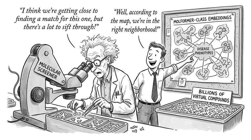
Recursion Pharmaceuticals uses molecular foundation models (including MolFormer-class embeddings) to screen billions of virtual compounds against disease-relevant cellular phenotypes. By embedding candidate molecules into a learned representation space and comparing them to embeddings of known active compounds, their platform reportedly identifies hit molecules up to 100 times faster than traditional high-throughput screening . This embedding-based virtual screen contributed to advancing multiple candidates into clinical trials, including treatments for rare genetic diseases where traditional screening would be prohibitively expensive.
Lab: Protein Embedding Explorer
Goal: Investigate how ESM-2 embeddings capture protein family membership by embedding, clustering, and visualizing 30+ protein sequences from three distinct families.
Tools needed: Python with transformers, torch, scikit-learn, umap-learn, and matplotlib. A GPU is helpful but the 8M-parameter ESM-2 checkpoint (facebook/esm2_t6_8M_UR50D) runs on CPU.
Procedure: (1) Retrieve 10 sequences each from three UniProt families: globins (e.g., hemoglobin/myoglobin), serine proteases (e.g., trypsin/chymotrypsin), and kinases (e.g., CDK2/EGFR). (2) Extract mean-pooled embeddings with ESM-2. (3) Reduce to 2D with UMAP and color-code by family. (4) Compute silhouette score, a measure of how well each point fits its assigned cluster versus the nearest alternative cluster , to quantify cluster separation.
What to vary: Switch between the 8M and 650M checkpoints and compare silhouette scores. Try using the embedding from different transformer layers (early, middle, final) to see which layer best separates families.
What to observe: The 650M model should produce tighter, more separated clusters. Middle-to-late layers tend to outperform the final layer for family-level similarity in many reported benchmarks, likely because the last layer specializes for the MLM prediction head rather than general representation .
Exercises
Exercise 27.4 (Conceptual): Compare the masked language modeling objective (ESM-2) with the autoregressive objective (ProGen2). What are the inductive biases of each? Why is masked modeling preferred for representation learning while autoregressive modeling is preferred for generation?
Exercise 27.5 (Coding): Using MolFormer, compute embeddings for a set of 20 common drug molecules. Cluster them using k-means (from Chapter 25) and visualize the clusters with UMAP (from Chapter 26). Do the clusters correspond to known drug classes (e.g., NSAIDs, antibiotics, antihistamines)?
Exercise 27.6 (Analysis): Download ESM-2 at two different sizes (8M and 650M parameters). Compute embeddings for the same 100 proteins and train a simple linear classifier for subcellular localization on each set of embeddings. Quantify the accuracy improvement from scaling and discuss whether it follows the scaling laws from Section 27.1.