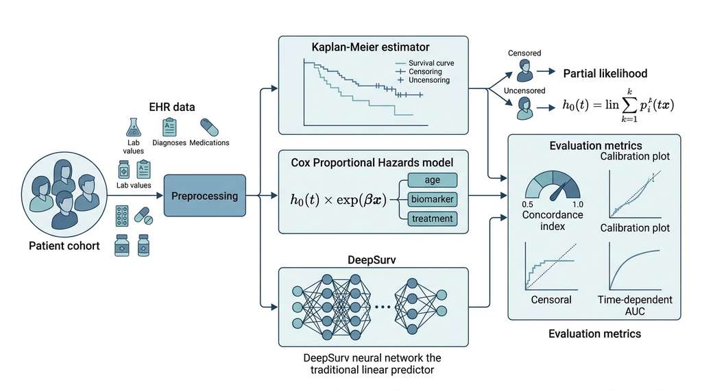
Clinical AI operates at the boundary between computational prediction and human health. Unlike protein folding or virtual screening, clinical models must contend with incomplete data, ethical constraints, regulatory requirements, and the irreducible uncertainty of human biology. The foundational tool is survival analysis, which models time-to-event outcomes (death, disease recurrence, treatment response) in the presence of censoring: patients who leave a study, have not yet experienced the event, or die from unrelated causes. This section builds from the classic Cox proportional hazards model through modern deep survival models, then addresses clinical trial design and biomarker discovery. Figure 48.7 illustrates how these components connect in a typical clinical AI pipeline.
1. Survival Analysis Fundamentals
A clinical trial enrolls 400 patients, but after three years only 210 have experienced the outcome the researchers are tracking; the rest moved, switched providers, or simply outlived the study window. Throwing away those 190 "incomplete" records would bias every conclusion, yet standard regression has no way to use them. Survival analysis solves this problem by modeling the time \(T\) until an event of interest occurs (death, relapse, treatment failure). It extracts information from every patient, including those whose outcome remains unknown. The key challenge is censoring: for some patients, researchers observe only that the event has not occurred by a certain time, not the actual event time. Right-censoring is the most common type: a patient who is alive at the end of the study contributes the information "survived at least this long" but not the actual survival time.
Survival analysis encompasses statistical methods designed for time-to-event data where some observations are incomplete (censored). It matters because standard regression treats "patient alive at study end" and "patient lost to follow-up at month 6" as identical missing values. Both discard the partial information each carries about how long the patient survived. The core mechanism is a likelihood function that splits each patient into one of two cases. Observed events contribute the probability of failing at the exact observed time. Censored observations contribute only the probability of surviving up to their last known time point. Use survival analysis whenever the outcome is "time until something happens" and some subjects have not yet experienced that event. Use standard classification when the outcome is a binary label observed for every subject at a fixed time horizon (e.g., "readmitted within 30 days, yes or no"). In short: survival analysis turns "we lost track of the patient" from a reason to discard data into a source of evidence.
Survival, Hazard, and Cumulative Hazard
Three equivalent functions describe the survival distribution:
The survival function \(S(t) = P(T > t)\) gives the probability of surviving beyond time \(t\). The hazard function $h(t) = \lim_{\Delta t \to 0} \frac{P(t \leq T < t + \Delta t \mid T \geq t)}{\Delta t}$ gives the instantaneous rate of the event at time \(t\), conditional on survival to that point. The cumulative hazard \(H(t) = \int_0^t h(u)\, du\) connects to the survival function via \(S(t) = \exp(-H(t))\).
Mental Model
Think of the hazard function like a dripping faucet with variable water pressure. The survival function tracks how full the bucket still is (the fraction of patients who have not yet experienced the event). The hazard function is the drip rate at each moment: how fast the bucket is losing water right now, given how much remains. A constant drip rate (constant hazard) means the faucet does not care how long it has been dripping; this is the exponential survival model. The Cox model says that each patient has their own faucet whose drip rate is the baseline rate multiplied by a patient-specific factor (determined by age, biomarkers, treatment). Crucially, the proportional hazards assumption means every patient's drip rate speeds up and slows down at the same times; only the multiplier differs. When that assumption breaks (e.g., a drug works well early but wears off), the faucets no longer move in lockstep, and you need a model like DeepHit that allows each patient's drip pattern to have its own shape over time.
1.1 The Kaplan-Meier Estimator
The Kaplan-Meier estimator is the nonparametric maximum likelihood estimate of the survival function. At each observed event time \(t_j\) with \(d_j\) events and \(n_j\) individuals at risk:
$$\hat{S}(t) = \prod_{t_j \leq t} \left(1 - \frac{d_j}{n_j}\right)$$import numpy as np
import pandas as pd
from lifelines import KaplanMeierFitter, CoxPHFitter
from lifelines.statistics import logrank_test
def kaplan_meier_analysis(
durations: np.ndarray,
events: np.ndarray,
groups: np.ndarray = None,
group_labels: list[str] = None,
) -> dict:
"""Kaplan-Meier survival analysis with optional group comparison.
Args:
durations: time-to-event or time-to-censoring for each patient
events: 1 if event observed, 0 if censored
groups: optional group assignments for stratified analysis
group_labels: names for the groups
Returns: fitted KM models and log-rank test results
"""
results = {}
if groups is None:
# Single-group analysis
kmf = KaplanMeierFitter()
kmf.fit(durations, event_observed=events)
results["median_survival"] = kmf.median_survival_time_
results["survival_at_12m"] = float(kmf.predict(12.0))
results["survival_at_24m"] = float(kmf.predict(24.0))
results["model"] = kmf
else:
# Stratified analysis with log-rank test
unique_groups = np.unique(groups)
models = {}
for g in unique_groups:
mask = groups == g
label = group_labels[int(g)] if group_labels else str(g)
kmf = KaplanMeierFitter()
kmf.fit(durations[mask], event_observed=events[mask], label=label)
models[label] = kmf
results["models"] = models
# Log-rank test between groups
if len(unique_groups) == 2:
mask1 = groups == unique_groups[0]
mask2 = groups == unique_groups[1]
lr = logrank_test(
durations[mask1], durations[mask2],
events[mask1], events[mask2],
)
results["logrank_p"] = lr.p_value
results["logrank_statistic"] = lr.test_statistic
return resultsCensoring is not missing data; it is a form of partial information. A censored observation tells you that the patient survived at least until the censoring time. Ignoring censored observations (analyzing only patients who experienced the event) introduces severe bias, because patients with longer survival times are more likely to be censored by end-of-study. Every survival model must properly handle censoring; standard regression and classification models cannot.
2. Cox Proportional Hazards
When an oncologist asks "does this biomarker predict shorter survival, and by how much?", the answer has historically flowed through a single model. Regulatory submissions to the FDA frequently cite it; clinical guidelines are built on its output; misspecifying it can mask a real treatment effect or manufacture a false one.
The Cox proportional hazards model is the workhorse of clinical survival analysis. It models the hazard for patient \(i\) as a function of covariates \(\mathbf{x}_i\) (age, biomarkers, treatment, genomic features):
$$h(t \mid \mathbf{x}_i) = h_0(t) \cdot \exp(\boldsymbol{\beta}^T \mathbf{x}_i)$$where \(h_0(t)\) is the baseline hazard (a nonparametric function of time shared by all patients) and \(\boldsymbol{\beta}\) are the regression coefficients. The model is "semi-parametric" (meaning it combines a parametric component, the covariate coefficients \(\boldsymbol{\beta}\), with a nonparametric component, the baseline hazard \(h_0(t)\), which is left completely unspecified).
The proportional hazards assumption means that the hazard ratio between any two patients is constant over time:
$$\frac{h(t \mid \mathbf{x}_i)}{h(t \mid \mathbf{x}_j)} = \exp\bigl(\boldsymbol{\beta}^T (\mathbf{x}_i - \mathbf{x}_j)\bigr)$$This ratio does not depend on \(t\) or \(h_0(t)\), which is why the baseline hazard cancels in the partial likelihood used for estimation.
2.1 The Partial Likelihood
Cox's key insight: the coefficients \(\boldsymbol{\beta}\) can be estimated without specifying \(h_0(t)\), using the partial likelihood. At each event time \(t_j\) where patient \(j\) experiences the event, the probability that it was patient \(j\) (rather than any other at-risk patient) is:
$$L_j(\boldsymbol{\beta}) = \frac{\exp(\boldsymbol{\beta}^T \mathbf{x}_j)}{\sum_{k \in \mathcal{R}(t_j)} \exp(\boldsymbol{\beta}^T \mathbf{x}_k)}$$where \(\mathcal{R}(t_j)\) is the risk set (all patients still under observation at time \(t_j\)). The full partial likelihood is the product over all event times:
$$L(\boldsymbol{\beta}) = \prod_{j: \delta_j = 1} \frac{\exp(\boldsymbol{\beta}^T \mathbf{x}_j)}{\sum_{k \in \mathcal{R}(t_j)} \exp(\boldsymbol{\beta}^T \mathbf{x}_k)}$$where \(\delta_j = 1\) indicates an observed event (not censored). Maximizing this partial likelihood yields the coefficient estimates \(\hat{\boldsymbol{\beta}}\).
import pandas as pd
import numpy as np
from lifelines import CoxPHFitter

def fit_cox_model(
    df: pd.DataFrame,
    duration_col: str = "time",
    event_col: str = "event",
    covariate_cols: list[str] = None,
    penalizer: float = 0.01,
) -> dict:
    """Fit a Cox proportional hazards model.

    Args:
        df: DataFrame with duration, event, and covariate columns
        duration_col: column with time-to-event values
        event_col: column with event indicators (1=event, 0=censored)
        covariate_cols: list of covariate column names
        penalizer: L2 regularization strength (prevents overfitting
            with many covariates)

    Returns: fitted model with coefficients, hazard ratios, and metrics
    """
    if covariate_cols is not None:
        cols = [duration_col, event_col] + covariate_cols
        df_model = df[cols].copy()
    else:
        df_model = df.copy()

    # Fit Cox model
    cph = CoxPHFitter(penalizer=penalizer)
    cph.fit(df_model, duration_col=duration_col, event_col=event_col)

    # Extract results
    summary = cph.summary
    results = {
        "concordance_index": cph.concordance_index_,
        "log_likelihood": cph.log_likelihood_,
        "aic": cph.AIC_partial_,
        "coefficients": {},
    }

    for covariate in summary.index:
        results["coefficients"][covariate] = {
            "coef": float(summary.loc[covariate, "coef"]),
            "hazard_ratio": float(summary.loc[covariate, "exp(coef)"]),
            "p_value": float(summary.loc[covariate, "p"]),
            "ci_lower": float(summary.loc[covariate, "exp(coef) lower 95%"]),
            "ci_upper": float(summary.loc[covariate, "exp(coef) upper 95%"]),
        }

    return results


def check_proportional_hazards(cph: CoxPHFitter, df: pd.DataFrame) -> dict:
    """Test the proportional hazards assumption.

    Uses Schoenfeld residuals to test whether covariate effects
    are constant over time. A significant p-value indicates
    violation of the PH assumption for that covariate.
    """
    ph_test = cph.check_assumptions(df, p_value_threshold=0.05, show_plots=False)
return ph_test2.2 The Concordance Index
The concordance index (C-index) is the standard metric for evaluating survival model discrimination. It measures the probability that, for a random pair of patients where one experienced the event earlier, the model assigns a higher risk score to the patient with the earlier event:
$$C = P(\hat{r}_i > \hat{r}_j \mid T_i < T_j, \delta_i = 1)$$where \(\hat{r}_i\) is the predicted risk score and \(T_i\) is the observed time. A C-index of 0.5 indicates random prediction; 0.7 to 0.8 is typical in practice for clinical models; above 0.8 is generally considered excellent, though the achievable range depends heavily on the prediction task and patient population.
Common Misconception
A high concordance index does not mean the model's predicted probabilities are accurate. The C-index measures only discrimination (can the model rank patients correctly?) and says nothing about calibration (are the predicted survival probabilities close to the true probabilities?). A model can achieve a C-index of 0.85 while systematically overestimating or underestimating survival by 20%. Always pair the C-index with calibration assessment, such as the Brier score, where the Brier score is the mean squared difference between predicted survival probabilities and observed binary outcomes at a given time horizon, providing a combined measure of discrimination and calibration. Calibration plots that compare predicted versus observed survival at specific time horizons are also essential.
from lifelines.utils import concordance_index

def evaluate_survival_model(
    predicted_risk: np.ndarray,
    durations: np.ndarray,
    events: np.ndarray,
    time_horizons: list[float] = None,
) -> dict:
    """Evaluate a survival prediction model.

    Metrics:
    - Concordance index (discrimination)
    - Time-dependent AUC at specific horizons
    - Brier score (calibration + discrimination)
    """
    # Overall concordance index
    c_index = concordance_index(durations, -predicted_risk, events)

    results = {"concordance_index": c_index}

    # Time-dependent evaluation at specific horizons
    if time_horizons is not None:
        from sksurv.metrics import cumulative_dynamic_auc, brier_score
        import numpy as np

        # Convert to structured array for scikit-survival
        y = np.array(
            [(bool(e), t) for e, t in zip(events, durations)],
            dtype=[("event", bool), ("time", float)],
        )

        for horizon in time_horizons:
            try:
                auc, mean_auc = cumulative_dynamic_auc(
                    y, y, predicted_risk, [horizon]
                )
                results[f"auc_at_{horizon}m"] = float(mean_auc)
            except Exception:
                pass

return resultsStep-Through: Cox Partial Likelihood Calculation
Trace through the partial likelihood with three patients. Patient A: event at month 4, covariates give \(\boldsymbol{\beta}^T \mathbf{x}_A = 0.8\). Patient B: censored at month 6, \(\boldsymbol{\beta}^T \mathbf{x}_B = 0.3\). Patient C: event at month 9, \(\boldsymbol{\beta}^T \mathbf{x}_C = -0.2\).
Event at month 4 (Patient A): Risk set = {A, B, C} (all alive). Contribution = $\exp(0.8) / [\exp(0.8) + \exp(0.3) + \exp(-0.2)] = 2.226 / [2.226 + 1.350 + 0.819] = 2.226 / 4.395 = 0.507$.
Month 6 (Patient B): Censored, so B contributes no numerator term. B simply drops out of future risk sets.
Event at month 9 (Patient C): Risk set = {C} (B was censored, A already had event). Contribution = \(\exp(-0.2) / \exp(-0.2) = 1.0\).
Partial likelihood: \(L = 0.507 \times 1.0 = 0.507\). Log partial likelihood = \(\ln(0.507) = -0.679\). The optimizer adjusts \(\boldsymbol{\beta}\) to maximize this value across all event times.
3. Deep Survival Models
The Cox model assumes a linear log-hazard: \(\log h(t | \mathbf{x}) = \log h_0(t) + \boldsymbol{\beta}^T \mathbf{x}\). When the relationship between a covariate and risk is nonlinear (for example, moderate blood pressure may increase risk only slightly while extreme values increase it dramatically), the linear model cannot capture this without manual feature engineering. Deep survival models relax the linearity constraint to learn nonlinear risk functions while preserving proper handling of censoring:
DeepSurv replaces the linear predictor with a neural network: \(h(t | \mathbf{x}) = h_0(t) \cdot \exp(f_\theta(\mathbf{x}))\). The loss function is the negative log partial likelihood, identical to the Cox model but with \(f_\theta(\mathbf{x})\) in place of \(\boldsymbol{\beta}^T \mathbf{x}\).
DeepHit models the full survival distribution without the proportional hazards assumption. It divides time into discrete intervals and predicts the probability of the event in each interval: \(P(T = t_k | \mathbf{x}) = f_\theta(\mathbf{x})_k\). The loss combines a log-likelihood term with a ranking loss (a penalty that increases when the model assigns a lower risk score to a patient who experienced the event earlier than another patient, encouraging correct pairwise ordering). As of 2024, transformer-based survival models such as SurvTRACE (Wang and Sun, 2022) extend these ideas by applying self-attention across both feature interactions and competing risks, in several benchmark comparisons matching or exceeding DeepHit on datasets like SUPPORT and METABRIC. Figure 48.4.1 illustrates the Cox proportional hazards model and deep survival models pipeline.
Checkpoint
So far: the Cox model handles censoring with a linear risk function, DeepSurv extends it to nonlinear risks via neural networks while keeping the proportional hazards assumption, and DeepHit removes that assumption entirely by modeling the full discrete-time survival distribution.
import torch
import torch.nn as nn

class DeepSurv(nn.Module):
    """DeepSurv: neural network Cox proportional hazards model.

    Replaces the linear predictor in Cox PH with a deep network
    while preserving the partial likelihood loss and proper
    handling of censoring.
    """

    def __init__(self, input_dim: int, hidden_dims: list[int] = None, dropout: float = 0.3):
        super().__init__()
        if hidden_dims is None:
            hidden_dims = [256, 128, 64]

        layers = []
        prev_dim = input_dim
        for h_dim in hidden_dims:
            layers.extend([
                nn.Linear(prev_dim, h_dim),
                nn.BatchNorm1d(h_dim),
                nn.ReLU(),
                nn.Dropout(dropout),
            ])
            prev_dim = h_dim
        layers.append(nn.Linear(prev_dim, 1))

        self.network = nn.Sequential(*layers)

    def forward(self, x: torch.Tensor) -> torch.Tensor:
        """Compute log-risk score for each patient."""
        return self.network(x).squeeze(-1)


def cox_partial_likelihood_loss(
    log_risk: torch.Tensor,
    durations: torch.Tensor,
    events: torch.Tensor,
) -> torch.Tensor:
    """Negative log partial likelihood for Cox PH models.

    Properly handles censoring: only patients with observed
    events contribute to the numerator; all at-risk patients
    contribute to the denominator.
    """
    # Sort by duration (descending for cumulative sum trick)
    sorted_indices = torch.argsort(durations, descending=True)
    log_risk = log_risk[sorted_indices]
    events = events[sorted_indices]

    # Log-sum-exp over risk set (cumulative sum in sorted order)
    log_cumsum_risk = torch.logcumsumexp(log_risk, dim=0)

    # Partial likelihood: sum over events only
    event_mask = events.bool()
    partial_ll = log_risk[event_mask] - log_cumsum_risk[event_mask]

    return -partial_ll.mean()


def train_deepsurv(
    model: DeepSurv,
    X_train: np.ndarray,
    durations_train: np.ndarray,
    events_train: np.ndarray,
    X_val: np.ndarray,
    durations_val: np.ndarray,
    events_val: np.ndarray,
    n_epochs: int = 200,
    lr: float = 1e-3,
    batch_size: int = 256,
) -> dict:
    """Train DeepSurv with early stopping on validation C-index."""
    optimizer = torch.optim.Adam(model.parameters(), lr=lr, weight_decay=1e-4)
    scheduler = torch.optim.lr_scheduler.ReduceLROnPlateau(
        optimizer, patience=10, factor=0.5
    )

    X_t = torch.tensor(X_train, dtype=torch.float32)
    dur_t = torch.tensor(durations_train, dtype=torch.float32)
    evt_t = torch.tensor(events_train, dtype=torch.float32)

    best_c_index = 0.0
    best_state = None

    for epoch in range(n_epochs):
        model.train()
        # Mini-batch training
        indices = torch.randperm(len(X_t))
        epoch_loss = 0.0
        n_batches = 0

        for start in range(0, len(X_t), batch_size):
            batch_idx = indices[start:start + batch_size]
            log_risk = model(X_t[batch_idx])
            loss = cox_partial_likelihood_loss(
                log_risk, dur_t[batch_idx], evt_t[batch_idx]
            )
            optimizer.zero_grad()
            loss.backward()
            optimizer.step()
            epoch_loss += loss.item()
            n_batches += 1

        # Validation
        model.eval()
        with torch.no_grad():
            val_risk = model(torch.tensor(X_val, dtype=torch.float32)).numpy()
        c_idx = concordance_index(durations_val, -val_risk, events_val)
        scheduler.step(-c_idx)

        if c_idx > best_c_index:
            best_c_index = c_idx
            best_state = model.state_dict().copy()

    model.load_state_dict(best_state)
return {"best_c_index": best_c_index}For standard survival analysis without implementing custom models, lifelines provides a complete toolkit in a few lines:
from lifelines import CoxPHFitter, WeibullAFTFitter

# Cox model in 3 lines
cph = CoxPHFitter(penalizer=0.01)
cph.fit(df, duration_col="time", event_col="event")
cph.print_summary()  # Coefficients, HRs, p-values, C-index

# Predict survival curves for new patients
survival_curves = cph.predict_survival_function(new_patients)
median_survival = cph.predict_median(new_patients)
predict_survival_function method returns a DataFrame of survival probabilities over time for each new patient.For more advanced needs (time-dependent AUC, integrated Brier score, random survival forests), scikit-survival extends the scikit-learn API to survival data, reducing hundreds of lines of custom evaluation code to standard sklearn-style fit/predict/score calls.
4. Risk Prediction from Electronic Health Records
The survival models above assume a clean input matrix of covariates, but real clinical data arrives in a far messier form: the electronic health record.
Electronic health records (EHRs) store longitudinal patient data: diagnoses, medications, lab results, procedures, and clinical notes. AI risk models predict outcomes from this data, including 30-day readmission, disease progression, and mortality. Three properties make EHR data difficult: it is temporal, irregularly sampled, and heterogeneous, mixing categorical codes, continuous lab values, and free text.
Research Frontier
Health-LLM (Google Research, 2024) and MOTOR (Steinberg et al., NeurIPS 2023) represent a shift toward foundation models for clinical prediction. MOTOR pre-trains a transformer on approximately 55 million patient timelines using a novel "Multi-Objective Temporal Outcome Regression" objective, learning to predict lab values, diagnoses, and procedures simultaneously across time. On downstream tasks (30-day readmission, in-hospital mortality, long-term survival), MOTOR has been reported to match or exceed task-specific models while requiring as few as 1% of the labeled examples for fine-tuning. This pre-train-then-fine-tune paradigm parallels the success of language model pre-training: the model learns temporal clinical dynamics from unlabeled EHR sequences and transfers that knowledge to specific prediction tasks, reducing the labeled data bottleneck that has historically limited clinical AI deployment.
import torch
import torch.nn as nn

class TemporalEHRModel(nn.Module):
    """Transformer-based risk prediction from EHR event sequences.

    Processes a patient's medical history as a sequence of
    (event_code, timestamp, value) tuples using a temporal
    transformer with time-aware positional encoding.
    """

    def __init__(
        self,
        vocab_size: int,        # Number of unique medical codes
        d_model: int = 128,
        n_heads: int = 4,
        n_layers: int = 3,
        max_events: int = 512,
        n_outcomes: int = 1,
    ):
        super().__init__()

        self.code_embedding = nn.Embedding(vocab_size, d_model)
        self.value_projection = nn.Linear(1, d_model)
        self.time_projection = nn.Linear(1, d_model)

        encoder_layer = nn.TransformerEncoderLayer(
            d_model=d_model,
            nhead=n_heads,
            dim_feedforward=d_model * 4,
            dropout=0.1,
            batch_first=True,
        )
        self.transformer = nn.TransformerEncoder(
            encoder_layer, num_layers=n_layers
        )

        self.output_head = nn.Sequential(
            nn.Linear(d_model, d_model // 2),
            nn.ReLU(),
            nn.Dropout(0.1),
            nn.Linear(d_model // 2, n_outcomes),
        )

    def forward(
        self,
        event_codes: torch.Tensor,    # (batch, seq_len) int
        event_times: torch.Tensor,    # (batch, seq_len) float (days)
        event_values: torch.Tensor,   # (batch, seq_len) float
        mask: torch.Tensor = None,    # (batch, seq_len) bool
    ) -> torch.Tensor:
        """Predict risk score from patient event history."""
        # Embed event codes
        code_emb = self.code_embedding(event_codes)

        # Project continuous values and timestamps
        time_emb = self.time_projection(event_times.unsqueeze(-1))
        value_emb = self.value_projection(event_values.unsqueeze(-1))

        # Combine embeddings
        x = code_emb + time_emb + value_emb

        # Apply transformer with causal masking
        if mask is not None:
            x = self.transformer(x, src_key_padding_mask=~mask)
        else:
            x = self.transformer(x)

        # Pool over sequence and predict
        if mask is not None:
            x = (x * mask.unsqueeze(-1)).sum(dim=1) / mask.sum(dim=1, keepdim=True)
        else:
            x = x.mean(dim=1)

return self.output_head(x).squeeze(-1)Real-World Application: Sepsis Early Warning
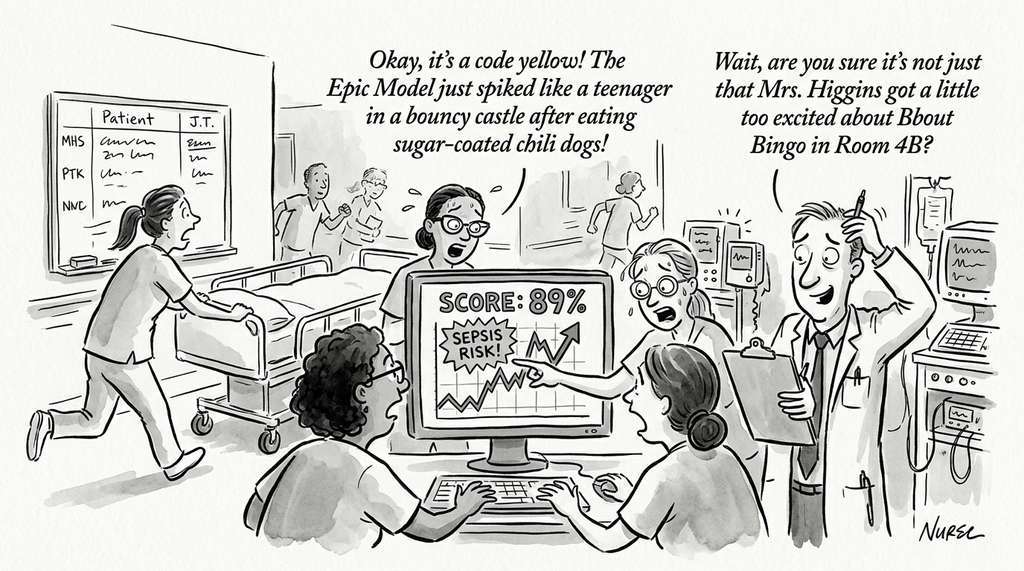
Epic Systems deploys a survival-style risk model called the Epic Sepsis Model across hundreds of U.S. hospitals. The system ingests EHR data (vital signs, lab results, nursing assessments) in real time and produces a time-varying risk score that triggers clinical alerts when sepsis probability crosses a threshold. Epic reported a C-index around 0.76, though an independent external validation (Wong et al., 2021) found substantially lower discrimination in practice. A key design lesson: the model's clinical utility depends less on its C-index and more on how alerts integrate into nursing workflows, because a perfectly discriminating model that fires too many false alarms gets ignored. As of 2024, several health systems have replaced or supplemented the Epic Sepsis Model with locally trained models that better reflect site-specific patient populations and workflow patterns.
The Ghost Patients Who Improved Predictions
When Google Health built a deep learning model for hospital readmission prediction (Rajkomar et al., 2018), they discovered that one of the strongest predictive features was the number of minutes between a patient's arrival at the emergency department and their first lab order. This "time to first lab" was not a biological signal at all; it was a proxy for how sick the triage nurse thought the patient looked. Sicker-looking patients got labs ordered faster. The model had, in effect, learned to read the nurse's clinical intuition through the timestamp metadata, a phenomenon researchers call "label leakage through clinical workflow." This finding sparked an ongoing debate about whether such features should be kept (they genuinely predict outcomes) or removed (they encode subjective judgment and may embed demographic biases in triage speed).
5. Clinical Trial Design
Predicting which patients are at risk is only half the problem; the other half is proving that a proposed treatment actually changes that risk, which is the job of the clinical trial.
Clinical trials are among the most expensive experiments in science: a Phase III (the large-scale confirmatory stage of drug testing, typically involving hundreds to thousands of patients) oncology trial typically costs \$50 million to \$200 million and takes 3 to 5 years. AI contributes to trial design in three ways:
5.1 Patient Stratification
Many drugs work well for a subset of patients and poorly for the rest. Biomarker-guided stratification identifies the responsive subpopulation before the trial begins, increasing the probability of detecting a treatment effect. The Cox model provides the mathematical framework: interaction terms (product terms that multiply treatment assignment by biomarker values, capturing how the treatment effect varies across biomarker levels) reveal differential treatment effects.
5.2 Adaptive Trial Design
Adaptive trials modify enrollment criteria, dosing, or even the primary endpoint during the trial based on interim results. Bayesian adaptive designs use the posterior probability (the updated belief about the treatment effect after observing interim data, as detailed in Chapter 32) to make stopping decisions:
$$P(\text{treatment effective} \mid \text{interim data}) > \theta_{\text{futility}}$$If the posterior probability drops below a futility threshold, the trial stops early, saving resources. If it exceeds an efficacy threshold, the trial may conclude early with a positive result. The Bayesian methods from Chapter 32 provide the mathematical foundation, and the experiment design framework from Chapter 46 formalizes the sequential decision-making.
import numpy as np
from scipy import stats

def simulate_adaptive_trial(
    n_max: int = 500,
    interim_analyses: list[int] = None,
    true_hazard_ratio: float = 0.75,
    futility_threshold: float = 0.10,
    efficacy_threshold: float = 0.99,
    n_simulations: int = 10000,
) -> dict:
    """Simulate a Bayesian adaptive clinical trial.

    Uses a Beta-Binomial model for simplicity (in practice,
    survival endpoints use more complex models).

    Args:
        n_max: maximum enrollment
        interim_analyses: patient counts at which to evaluate
        true_hazard_ratio: true treatment effect (< 1 = beneficial)
        futility_threshold: stop if P(effective) < this
        efficacy_threshold: stop if P(effective) > this
        n_simulations: number of trial simulations
    """
    if interim_analyses is None:
        interim_analyses = [100, 200, 300, 400]

    # Convert HR to response probability difference
    p_control = 0.30  # Baseline response rate
    p_treatment = 1 - (1 - p_control) ** true_hazard_ratio

    results = {
        "stopped_early_futility": 0,
        "stopped_early_efficacy": 0,
        "completed": 0,
        "true_positive": 0,
        "average_enrollment": 0,
    }

    for _ in range(n_simulations):
        # Simulate patient outcomes
        treatment_responses = np.random.binomial(1, p_treatment, n_max)
        control_responses = np.random.binomial(1, p_control, n_max)

        stopped = False
        for n_interim in interim_analyses:
            n_per_arm = n_interim // 2

            # Observed responses
            r_t = treatment_responses[:n_per_arm].sum()
            r_c = control_responses[:n_per_arm].sum()

            # Bayesian posterior: Beta(1 + successes, 1 + failures)
            # P(treatment > control)
            n_mc = 10000
            post_t = stats.beta.rvs(1 + r_t, 1 + n_per_arm - r_t, size=n_mc)
            post_c = stats.beta.rvs(1 + r_c, 1 + n_per_arm - r_c, size=n_mc)
            p_effective = (post_t > post_c).mean()

            if p_effective < futility_threshold:
                results["stopped_early_futility"] += 1
                results["average_enrollment"] += n_interim
                stopped = True
                break
            elif p_effective > efficacy_threshold:
                results["stopped_early_efficacy"] += 1
                results["true_positive"] += 1
                results["average_enrollment"] += n_interim
                stopped = True
                break

        if not stopped:
            results["completed"] += 1
            results["average_enrollment"] += n_max

    # Normalize
    results["average_enrollment"] /= n_simulations
    for key in ["stopped_early_futility", "stopped_early_efficacy",
                "completed", "true_positive"]:
        results[key] /= n_simulations

return resultsThe I-SPY 2 breast cancer trial is a landmark adaptive platform trial that has been running since 2010. It uses Bayesian adaptive randomization to test multiple experimental drugs simultaneously against a common control arm. Drugs that show early promise receive more patients (adaptive randomization); drugs that appear ineffective are dropped (futility analysis). The trial uses biomarker-guided stratification, assigning patients to treatment arms based on hormone receptor status, Human Epidermal growth factor Receptor 2 (HER2) status, and MammaPrint genomic score, where MammaPrint is a 70-gene expression signature that classifies breast tumors into high-risk or low-risk categories for distant recurrence. As of 2025, I-SPY 2 has evaluated over 20 experimental arms and graduated approximately 7 drugs to Phase III trials (circa 2024), with an average time-to-decision of 2 to 3 years compared to 5 to 7 years in traditional designs.
5.3 Regulatory Considerations
Clinical AI models that inform treatment decisions or trial designs face regulatory scrutiny from agencies such as the FDA (United States), EMA (European Union), and PMDA (Japan). In the United States, the FDA's Software as a Medical Device (SaMD) framework classifies AI tools by the seriousness of the condition they address and whether they inform or drive clinical decisions. Models that provide decision support (flagging high-risk patients for physician review) typically face a lighter regulatory path than models that autonomously recommend treatment changes. Regulatory submissions generally require evidence of clinical validity (does the model predict the outcome accurately in diverse populations?), analytical validity (is the model reproducible across sites and data pipelines?), and ongoing performance monitoring after deployment, because patient populations and clinical workflows shift over time. The adaptive trial designs described above must also satisfy regulatory requirements for Type I error control, typically through pre-specified stopping boundaries and simulation-based operating characteristics that demonstrate the design maintains the intended false-positive rate.
6. Biomarker Discovery
Adaptive trials succeed when they enroll the right patients, and identifying the right patients requires knowing which biological signals distinguish responders from non-responders.
Biomarkers are measurable indicators of biological processes: genes whose expression level predicts drug response, proteins whose blood concentration indicates disease progression, or imaging features that predict treatment outcome. AI accelerates biomarker discovery by learning which features, among thousands of candidates, are most predictive of clinical outcomes.
The survival model framework provides a natural approach: fit a regularized Cox
model with all candidate biomarkers as covariates, and the features that receive
nonzero coefficients are biomarker candidates. L1 (lasso) regularization performs
feature selection automatically. The code below uses elastic net regularization, where elastic net is a combination of L1 (lasso) and L2 (ridge) penalties controlled by the l1_ratio parameter, balancing feature selection with coefficient stability:
from lifelines import CoxPHFitter

def discover_biomarkers(
    df: pd.DataFrame,
    duration_col: str = "time",
    event_col: str = "event",
    candidate_cols: list[str] = None,
    l1_ratio: float = 0.5,
    penalizer: float = 0.1,
    significance_threshold: float = 0.05,
) -> list[dict]:
    """Discover prognostic biomarkers using regularized Cox regression.

    Uses elastic net regularization (L1 + L2) to select a sparse
    set of biomarkers from many candidates. L1 drives most
    coefficients to zero; surviving features are biomarker candidates.
    """
    if candidate_cols is None:
        exclude = {duration_col, event_col}
        candidate_cols = [c for c in df.columns if c not in exclude]

    cols = [duration_col, event_col] + candidate_cols

    cph = CoxPHFitter(
        penalizer=penalizer,
        l1_ratio=l1_ratio,
    )
    cph.fit(df[cols], duration_col=duration_col, event_col=event_col)

    # Extract significant biomarkers
    summary = cph.summary
    biomarkers = []
    for feature in summary.index:
        coef = float(summary.loc[feature, "coef"])
        hr = float(summary.loc[feature, "exp(coef)"])
        p = float(summary.loc[feature, "p"])

        if abs(coef) > 1e-6:  # Non-zero after L1 regularization
            biomarkers.append({
                "feature": feature,
                "coefficient": coef,
                "hazard_ratio": hr,
                "p_value": p,
                "significant": p < significance_threshold,
                "direction": "risk" if hr > 1 else "protective",
            })

return sorted(biomarkers, key=lambda x: abs(x["coefficient"]), reverse=True)Biomarker discovery illustrates the tension between prediction and causation explored in Chapter 31. A gene expression level that predicts survival is a prognostic biomarker, but it is not necessarily a drug target. A gene that causes disease progression, identified through Mendelian randomization (where naturally occurring genetic variants serve as instrumental variables to estimate causal effects of modifiable exposures on disease outcomes) or experimental perturbation, is a causal biomarker and a valid target. The causal inference methods from Chapter 31, particularly instrumental variable analysis and mediation analysis, distinguish these cases. The single-cell perturbation models from Section 48.3 provide experimental evidence of causality at the cellular level.
7. Discovery Workbench Integration
The Discovery Workbench gains a ClinicalAnalyzer component that
provides survival analysis, biomarker discovery, and trial simulation capabilities.
The component accepts clinical datasets in standard formats, fits survival models
with automatic assumption checking, and logs all results for provenance tracking.
from discovery_workbench import Analyzer, ExperimentRegistry

class ClinicalAnalyzer(Analyzer):
    """Clinical analysis pipeline for the Discovery Workbench."""

    def survival_analysis(
        self,
        df: pd.DataFrame,
        covariates: list[str],
        duration_col: str = "time",
        event_col: str = "event",
    ) -> dict:
        """Full survival analysis with model selection and validation."""
        run_id = self.registry.start_run(pipeline="clinical_analysis")

        # Fit Cox model
        cox_results = fit_cox_model(df, duration_col, event_col, covariates)

        # Check proportional hazards assumption
        cph = CoxPHFitter(penalizer=0.01)
        cph.fit(df[[duration_col, event_col] + covariates],
                duration_col=duration_col, event_col=event_col)

        # Biomarker discovery
        biomarkers = discover_biomarkers(df, duration_col, event_col, covariates)

        self.registry.log_stage(run_id, "survival", {
            "c_index": cox_results["concordance_index"],
            "n_biomarkers": len([b for b in biomarkers if b["significant"]]),
        })
        self.registry.end_run(run_id)

        return {
            "cox_model": cox_results,
            "biomarkers": biomarkers,
}Try It: Survival Analysis on the GBSG2 Dataset
Build a complete survival analysis pipeline using the German Breast Cancer Study
Group (GBSG2) dataset, which is bundled with scikit-survival and requires no
download.
(1) Install dependencies: pip install lifelines scikit-survival matplotlib.
(2) Load the dataset and inspect it:
from sksurv.datasets import load_gbsg2; X, y = load_gbsg2().
Convert the structured array y into separate duration
and event arrays, and one-hot encode categorical covariates with
pd.get_dummies.
(3) Plot Kaplan-Meier curves stratified by hormone therapy
(horTh column) using lifelines.KaplanMeierFitter, and
run a log-rank test to check whether the survival difference is statistically
significant.
(4) Fit a Cox proportional hazards model on all covariates, print the summary
to identify which features have significant hazard ratios, and verify the
proportional hazards assumption with cph.check_assumptions().
(5) Split the data 70/30, fit the Cox model on the training set, and evaluate
the concordance index on the held-out test set. Compare this C-index against a
random survival forest from
sksurv.ensemble.RandomSurvivalForest to see whether nonlinear
modeling improves discrimination on this dataset.
Exercise 48.4.1
A clinical trial reports three patients. Patient 1: died at month 10. Patient 2: alive and censored at month 14. Patient 3: died at month 18. Using the Kaplan-Meier formula, compute \(\hat{S}(t)\) at each event time and determine the median survival time. Then explain: if Patient 2 had instead been censored at month 8 (before the first event), how would \(\hat{S}(10)\) change, and why?
Hint
At each event time \(t_j\), compute \(1 - d_j / n_j\) where \(n_j\) is the number still at risk (not yet experienced the event and not yet censored). The survival estimate is the running product of these terms. Censored patients reduce the risk set for subsequent event times but do not create a step in the survival curve. If Patient 2 is censored at month 8, the risk set at month 10 shrinks from 3 to 2, which changes the step size.
Lab: Survival Model Showdown on Real Clinical Data
Goal: Compare a Cox proportional hazards model against a random survival forest on the Veterans Administration lung cancer dataset, and determine whether nonlinear modeling improves discrimination for this cohort.
Tools: Python with lifelines, scikit-survival,
and matplotlib (install via pip install lifelines scikit-survival matplotlib).
Steps (20 minutes):
(1) Load the dataset: from sksurv.datasets import load_veterans_lung_cancer.
(2) Preprocess: one-hot encode the categorical columns (Celltype,
Prior_therapy, Treatment).
(3) Split 70/30 stratified by event status.
(4) Fit a CoxPHFitter on the training set and record the test C-index.
(5) Fit a RandomSurvivalForest(n_estimators=100) on the same split and
record its test C-index.
(6) Plot both predicted survival curves for a single high-risk patient overlaid on
one figure.
What to vary: Try adding L1 regularization to the Cox model
(l1_ratio=1.0, penalizer=0.1) and increasing forest depth
(max_depth=5 vs. unlimited). Observe which changes improve or degrade
the C-index, and whether the gap between linear and nonlinear models widens or
narrows.
What to observe: Does the random survival forest consistently beat
Cox, or does the small sample size (137 patients) limit the benefit of nonlinear
modeling? Check whether the Cox model's proportional hazards assumption holds using
cph.check_assumptions(); violations suggest the forest may capture
time-varying effects the Cox model misses.