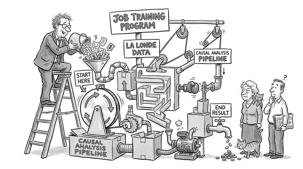
"I passed all four refutation tests, reported my effect with confidence intervals, and then my PI asked me to try a different DAG. I had 47 more candidates."
A Causal Graph With Too Many Confounders
Prerequisites
This section integrates everything from the chapter: the structural causal model formalism
(Section 31.1), causal discovery algorithms
(Section 31.2), and treatment effect estimation with
sensitivity analysis (Section 31.3). You should be
comfortable with DoWhy's four-step workflow, at least one causal discovery algorithm, and the
Conditional Average Treatment Effect (CATE) estimation methods. Familiarity with the Discovery Workbench architecture from
Chapter 6 will
help you understand the integration pattern.
The Big Picture
Individual causal tools are powerful, but real scientific workflows require them to work
together: explore data, discover plausible causal structures, estimate effects, test
robustness, and document every assumption. This section builds a complete causal analysis
pipeline that takes raw observational data and produces heterogeneous treatment effect
estimates with refutation-tested confidence intervals. The pipeline is modular: each stage
can be swapped independently (different discovery algorithm, different estimator, different
sensitivity analysis), and the entire workflow produces an auditable artifact that records
the causal graph, identification strategy, estimates, and refutation results. By the end,
you will have a reusable recipe for causal analysis that integrates into the Discovery
Workbench.
1. The Pipeline Architecture
A researcher hands you ten thousand field observations and asks: does a new soil treatment genuinely increase crop yield, or does it merely correlate with the rainfall patterns that drove both treatment decisions and harvests? Answering that question requires six coordinated stages. Each stage produces an intermediate artifact that feeds the next:
Data preparation and exploratory analysis: load data, check covariate balance, assess positivity (the requirement that every subgroup defined by covariates has a non-zero probability of receiving each treatment level), and identify potential confounders through domain knowledge and correlation analysis.
Causal graph specification: combine domain knowledge with causal discovery algorithms to construct a plausible directed acyclic graph (DAG). Run multiple algorithms and compare.
Identification: apply the backdoor criterion (a graphical test that determines whether conditioning on a set of variables blocks all non-causal paths between treatment and outcome), or alternatives such as the front-door criterion or instrumental variables, to determine the estimand and valid adjustment sets.
Estimation: compute Average Treatment Effect (ATE), Average Treatment on the Treated (ATT), and CATE using doubly robust estimators (methods that combine an outcome model and a treatment model so that the estimate remains consistent if either model is correctly specified) or Double Machine Learning (DML, a method that uses sample-splitting to separate nuisance parameter estimation from treatment effect estimation, reducing regularization bias) estimators. Compare multiple estimators as a robustness check.
Refutation and sensitivity: run placebo, random common cause, subset, and E-value tests (where the E-value quantifies the minimum strength an unmeasured confounder would need to fully explain away the observed effect). Flag estimates that fail any refutation.
Reporting: generate a structured report with the DAG, estimates, confidence intervals, refutation results, and a plain-language interpretation.
The pipeline targets a concrete scenario: estimating the heterogeneous effect of a soil
treatment on crop yield from observational data where environmental conditions confound
treatment assignment. In short: a causal pipeline turns "these two variables moved together" into "changing this one caused that one to move, and here is how much, for whom, and how confident we are."
Figure 31.6 illustrates how these six stages connect into a single end-to-end workflow.
Figure 31.6: The six-stage causal analysis pipeline. Data preparation feeds a causal graph (discovered or expert-specified), which is identified, estimated, refuted, and packaged into an auditable report artifact. Arrows indicate data flow; labels beneath each box name the intermediate artifact produced at that stage.
import numpy as np
import pandas as pd
from dataclasses import dataclass, field
from typing import Optional

@dataclass
class CausalPipelineConfig:
    """Configuration for a causal analysis pipeline run."""
    treatment: str
    outcome: str
    covariates: list[str]
    graph_spec: Optional[str] = None  # DOT string; None = discover from data
    discovery_algorithm: str = "pc"   # pc, fci, ges, lingam
    estimator: str = "dml"            # ipw, aipw, dml, t_learner, x_learner
    alpha: float = 0.05               # Significance level
    n_refutation_sims: int = 100      # Number of refutation simulations
    cross_fit_folds: int = 5          # DML cross-fitting folds

@dataclass
class CausalPipelineResult:
    """Structured output from a causal analysis pipeline run."""
    config: CausalPipelineConfig
    discovered_graph: Optional[object] = None
    identified_estimand: Optional[object] = None
    ate: float = 0.0
    ate_ci: tuple = (0.0, 0.0)
    att: float = 0.0
    cate_model: Optional[object] = None
    refutation_results: dict = field(default_factory=dict)
    e_value: float = 0.0
    passed_all_refutations: bool = False
Listing 31.18: Data classes for pipeline configuration and structured results. CausalPipelineConfig specifies the causal question (treatment, outcome, covariates) and methodological choices (discovery algorithm, estimator, cross-fitting fold count, where cross-fitting is the sample-splitting procedure DML uses to avoid overfitting the nuisance models). CausalPipelineResult captures every output artifact for auditing.
2. Data Preparation and Covariate Balance
Before any causal analysis, we need to understand the data. The critical pre-analysis checks
are: (a) covariate balance, the extent to which treated and control groups
differ on observed characteristics; (b) positivity, whether every combination
of covariate values has a non-zero probability of receiving each treatment; and
(c) missing data patterns, which can introduce selection bias if missingness
is related to treatment or outcome.
Covariate balance measures how similar the treated and control groups are on each variable before statistical adjustment. Large imbalances signal confounding: if treated units differ systematically from controls on a variable that also affects the outcome, a naive comparison of group means produces biased estimates. The standard metric, the standardized mean difference (SMD), divides the difference in group means by the pooled standard deviation. Values above 0.1 flag meaningful imbalance. Use covariate balance as a first-pass diagnostic before choosing an adjustment strategy. When all SMDs fall below 0.05, simpler estimators such as regression adjustment may suffice. Severe imbalance on key confounders calls for propensity score methods (which model the probability of receiving treatment given covariates and use that probability to reweight or match observations) or doubly robust estimators that handle larger extrapolation.
Listing 31.19: Generating synthetic crop yield data with known confounding and assessing covariate balance via standardized mean differences. SMD values above 0.1 indicate meaningful imbalance requiring causal adjustment; rainfall and soil pH show imbalance because they drive treatment assignment in the data-generating process.
The covariate balance assessment reveals which variables differ between treated and control
groups, providing empirical evidence of confounding. Variables with large standardized mean
differences are candidates for the adjustment set. Note that balance on observed covariates
does not guarantee balance on unmeasured confounders; this is why sensitivity
analysis remains essential.
Once these balance diagnostics reveal which covariates differ between groups, the next question is how those variables relate to each other causally, a question that requires specifying the full structure of the data-generating process as a graph.
3. Causal Graph Discovery and Specification
The pipeline supports two modes for obtaining the causal graph: expert specification (the
researcher provides a DAG) and data-driven discovery (algorithms learn the skeleton and
orientations from data). In practice, the most effective approach combines both: start with
domain knowledge, use discovery algorithms to check consistency, and resolve disagreements
through discussion with domain experts.
from causallearn.search.ConstraintBased.PC import pc
from causallearn.search.ScoreBased.GES import ges
from causallearn.utils.cit import fisherz

def discover_causal_graph(data, covariates, treatment, outcome, method="pc"):
    """Run causal discovery and return a DOT string for DoWhy.

    Compares the data-driven graph with domain knowledge and
    flags inconsistencies.
    """
    all_vars = covariates + [treatment, outcome]
    analysis_data = data[all_vars].values
    labels = all_vars

    if method == "pc":
        result = pc(analysis_data, alpha=0.05, indep_test=fisherz,
                     node_names=labels)
        adj = result.G.graph
    elif method == "ges":
        result = ges(analysis_data, score_func="local_score_BIC")
        adj = result["G"].graph
    else:
        raise ValueError(f"Unknown method: {method}")

    # Extract edges from adjacency matrix
    edges = []
    for i in range(len(labels)):
        for j in range(len(labels)):
            if adj[i, j] == -1 and adj[j, i] == 1:
                edges.append((labels[i], labels[j]))

    print(f"\n{method.upper()} discovered edges:")
    for src, dst in edges:
        print(f"  {src} -> {dst}")

    return edges

# Run multiple discovery algorithms
pc_edges = discover_causal_graph(
    data, covariates, "treatment", "yield_kg", method="pc"
)
ges_edges = discover_causal_graph(
    data, covariates, "treatment", "yield_kg", method="ges"
)

# Compare: edges present in both algorithms are more trustworthy
pc_set = set(pc_edges)
ges_set = set(ges_edges)
consensus = pc_set & ges_set
pc_only = pc_set - ges_set
ges_only = ges_set - pc_set

print("\nConsensus edges (both algorithms agree):")
for edge in consensus:
    print(f"  {edge[0]} -> {edge[1]}")
if pc_only:
    print("PC-only edges:")
    for edge in pc_only:
        print(f"  {edge[0]} -> {edge[1]}")
if ges_only:
    print("GES-only edges:")
    for edge in ges_only:
        print(f"  {edge[0]} -> {edge[1]}")
Listing 31.20: Multi-algorithm causal discovery using PC (Peter-Clark, a constraint-based algorithm that removes edges via conditional independence tests) and GES (Greedy Equivalence Search, a score-based algorithm that greedily adds and removes edges to maximize a penalized likelihood score). Edges present in both outputs form a consensus set that receives higher confidence than edges found by only one method.
def build_causal_graph_dot(
    covariates, treatment, outcome,
    discovered_edges=None, domain_knowledge=None
) -> str:
    """Construct a DoWhy-compatible DOT graph string.

    Merges domain knowledge with discovered edges, preferring
    domain knowledge when they conflict.
    """
    # Default domain knowledge for crop yield
    if domain_knowledge is None:
        domain_knowledge = {
            ("rainfall", "treatment"),
            ("rainfall", "yield_kg"),
            ("soil_ph", "treatment"),
            ("soil_ph", "yield_kg"),
            ("temperature", "yield_kg"),
            ("treatment", "yield_kg"),
        }

    # Start with domain knowledge, add non-conflicting discovered edges
    final_edges = set(domain_knowledge)
    if discovered_edges:
        for edge in discovered_edges:
            reverse = (edge[1], edge[0])
            if reverse not in final_edges:
                final_edges.add(edge)

    # Build DOT string
    edge_lines = [f"    {src} -> {dst};" for src, dst in final_edges]
    dot = "digraph {\n" + "\n".join(edge_lines) + "\n}"

    print(f"\nFinal causal graph ({len(final_edges)} edges):")
    print(dot)
    return dot

graph_dot = build_causal_graph_dot(
    covariates, "treatment", "yield_kg",
    discovered_edges=list(consensus),
)
Listing 31.21: Merging domain knowledge with data-driven discovery into a final causal graph encoded as a DOT string (a plain-text graph description language used by Graphviz and accepted by DoWhy for specifying causal structures). Domain knowledge takes precedence when algorithms disagree; discovered edges supplement the expert-specified structure.
Key Insight: Domain Knowledge Is Not Cheating
Researchers sometimes worry that incorporating domain knowledge into causal discovery
"contaminates" a purely data-driven analysis. The opposite is true: ignoring domain
knowledge is the mistake. Causal discovery algorithms operate under strong assumptions
(faithfulness, which requires that every conditional independence in the data reflects a genuine structural separation in the graph,causal sufficiency, which assumes that all common causes of measured variables are also measured, and correct conditional independence tests) that can
fail in practice. Domain knowledge constrains the search space, prevents absurd graphs (rain
does not cause soil pH), and resolves equivalence class ambiguities that no algorithm can
break from observational data alone. The scientific question is not "what can the data tell
us without any prior knowledge?" but "what does the data tell us, given what we already know?"
This philosophy connects to the Bayesian
reasoning of Chapter 32, where prior knowledge is formalized as a prior distribution.
Checkpoint
So far: you have seen how to assess covariate balance with standardized mean differences, run multiple causal discovery algorithms to build a consensus graph, and merge data-driven edges with domain knowledge into a final DAG suitable for identification.
4. The Complete Pipeline
Without an integrated pipeline, teams routinely ship causal claims that pass one test but collapse under another: an estimate that looks stable in a subset check can still be an artifact of a misspecified graph, and a well-identified estimand can still yield nonsense if positivity is violated. Assembling each stage into a single, auditable workflow is what prevents these silent failures from reaching publication.
With the building blocks in place, we assemble the complete pipeline. The CausalAnalysisPipeline
class orchestrates data preparation, graph specification, identification, estimation, and
refutation into a single callable workflow, following the six stages shown in Figure 31.6.
import dowhy
from dowhy import CausalModel
from econml.dml import LinearDML, CausalForestDML
from sklearn.ensemble import (
    GradientBoostingRegressor, GradientBoostingClassifier
)

class CausalAnalysisPipeline:
    """End-to-end causal analysis: discover, identify, estimate, refute."""

    def __init__(self, config: CausalPipelineConfig):
        self.config = config
        self.result = CausalPipelineResult(config=config)

    def run(self, data: pd.DataFrame) -> CausalPipelineResult:
        """Execute the full pipeline."""
        print("=" * 60)
        print("CAUSAL ANALYSIS PIPELINE")
        print("=" * 60)

        # Stage 1: Data preparation
        print("\n--- Stage 1: Data Preparation ---")
        self._check_data(data)

        # Stage 2: Graph specification
        print("\n--- Stage 2: Causal Graph ---")
        graph_dot = self._get_graph(data)

        # Stage 3: Identification
        print("\n--- Stage 3: Identification ---")
        model = CausalModel(
            data=data,
            treatment=self.config.treatment,
            outcome=self.config.outcome,
            graph=graph_dot,
        )
        estimand = model.identify_effect(proceed_when_unidentifiable=True)  # warns rather than halting when no valid adjustment set exists, letting the analyst inspect the partial result
        self.result.identified_estimand = estimand
        print(f"Estimand type: {estimand.estimands}")

        # Stage 4: Estimation (ATE + CATE)
        print("\n--- Stage 4: Estimation ---")
        self._estimate_effects(data, model, estimand)

        # Stage 5: Refutation
        print("\n--- Stage 5: Refutation ---")
        self._run_refutations(model, estimand)

        # Stage 6: Summary
        print("\n--- Stage 6: Summary ---")
        self._print_summary()

        return self.result

    def _check_data(self, data):
        """Validate data and report basic diagnostics."""
        n = len(data)
        n_treated = data[self.config.treatment].sum()
        print(f"  Samples: {n}")
        print(f"  Treated: {n_treated} ({n_treated/n:.1%})")
        print(f"  Control: {n - n_treated} ({(n-n_treated)/n:.1%})")

        # Check positivity
        for cov in self.config.covariates:
            for quantile in [0.05, 0.95]:
                threshold = data[cov].quantile(quantile)
                if quantile < 0.5:
                    subset = data[data[cov] <= threshold]
                else:
                    subset = data[data[cov] >= threshold]
                treat_rate = subset[self.config.treatment].mean()
                if treat_rate < 0.02 or treat_rate > 0.98:


  Try It: End-to-End Causal Pipeline on Real-World Data

                    print(f"  WARNING: Positivity concern for {cov} "
                          f"at {quantile:.0%} quantile "
                          f"(treatment rate = {treat_rate:.1%})")

    def _get_graph(self, data):
        """Return or discover the causal graph."""
        if self.config.graph_spec:
            print("  Using expert-specified graph")
            return self.config.graph_spec

        print(f"  Discovering graph with {self.config.discovery_algorithm}")
        edges = discover_causal_graph(
            data, self.config.covariates,
            self.config.treatment, self.config.outcome,
            method=self.config.discovery_algorithm,
        )
        return build_causal_graph_dot(
            self.config.covariates,
            self.config.treatment,
            self.config.outcome,
            discovered_edges=edges,
        )

    def _estimate_effects(self, data, model, estimand):
        """Estimate ATE and CATE."""
        X = data[self.config.covariates].values
        T = data[self.config.treatment].values
        Y = data[self.config.outcome].values

        # ATE via DoWhy + DML
        estimate = model.estimate_effect(
            estimand,
            method_name="backdoor.econml.dml.DML",
            method_params={
                "init_params": {
                    "model_y": GradientBoostingRegressor(
                        n_estimators=200, max_depth=4, min_samples_leaf=20
                    ),
                    "model_t": GradientBoostingClassifier(
                        n_estimators=200, max_depth=4, min_samples_leaf=20
                    ),
                    "cv": self.config.cross_fit_folds,
                },
                "fit_params": {},
            },
        )

        self.result.ate = estimate.value
        self._dowhy_estimate = estimate
        print(f"  ATE: {estimate.value:.2f}")

        # CATE via CausalForestDML for heterogeneity
        # CausalForestDML extends DML by replacing the final-stage linear model
        # with a causal random forest, capturing nonlinear effect heterogeneity
        cate_model = CausalForestDML(
            model_y=GradientBoostingRegressor(
                n_estimators=200, max_depth=4, min_samples_leaf=20
            ),
            model_t=GradientBoostingClassifier(
                n_estimators=200, max_depth=4, min_samples_leaf=20
            ),
            cv=self.config.cross_fit_folds,
            n_estimators=500,
            random_state=42,
        )
        cate_model.fit(Y, T, X=X)
        self.result.cate_model = cate_model

        # CATE summary
        cate_pred = cate_model.effect(X)
        cate_intervals = cate_model.effect_interval(X, alpha=self.config.alpha)

        print(f"  CATE mean: {cate_pred.mean():.2f}")
        print(f"  CATE std:  {cate_pred.std():.2f}")
        print(f"  CATE range: [{cate_pred.min():.2f}, {cate_pred.max():.2f}]")

        # Store ATE CI from causal forest
        ate_from_forest = cate_model.ate()
        ate_ci = cate_model.ate_interval(alpha=self.config.alpha)
        self.result.ate_ci = (ate_ci[0], ate_ci[1])
        print(f"  ATE (forest): {ate_from_forest:.2f}")
        print(f"  95% CI: [{ate_ci[0]:.2f}, {ate_ci[1]:.2f}]")

    def _run_refutations(self, model, estimand):
        """Run all refutation tests."""
        estimate = self._dowhy_estimate
        all_passed = True

        # Placebo treatment
        try:
            ref_placebo = model.refute_estimate(
                estimand, estimate,
                method_name="placebo_treatment_refuter",
                placebo_type="permute",
                num_simulations=self.config.n_refutation_sims,
            )
            placebo_effect = ref_placebo.new_effect
            # 10% threshold is a common heuristic, not a universal standard;
            # adjust based on domain-specific tolerance for residual signal
            placebo_pass = abs(placebo_effect) < abs(estimate.value) * 0.1
            self.result.refutation_results["placebo"] = {
                "effect": placebo_effect,
                "passed": placebo_pass,
            }
            status = "PASS" if placebo_pass else "FAIL"
            print(f"  Placebo:        {status} (effect={placebo_effect:.3f})")
            if not placebo_pass:
                all_passed = False
        except Exception as e:
            print(f"  Placebo:        ERROR ({e})")
            all_passed = False

        # Random common cause
        try:
            ref_random = model.refute_estimate(
                estimand, estimate,
                method_name="random_common_cause",
                num_simulations=self.config.n_refutation_sims,
            )
            random_effect = ref_random.new_effect
            random_pass = abs(random_effect - estimate.value) < abs(estimate.value) * 0.1
            self.result.refutation_results["random_common_cause"] = {
                "effect": random_effect,
                "passed": random_pass,
            }
            status = "PASS" if random_pass else "FAIL"
            print(f"  Random cause:   {status} (effect={random_effect:.3f})")
            if not random_pass:
                all_passed = False
        except Exception as e:
            print(f"  Random cause:   ERROR ({e})")
            all_passed = False

        # Data subset
        try:
            ref_subset = model.refute_estimate(
                estimand, estimate,
                method_name="data_subset_refuter",
                subset_fraction=0.8,
                num_simulations=self.config.n_refutation_sims,
            )
            subset_effect = ref_subset.new_effect
            subset_pass = abs(subset_effect - estimate.value) < abs(estimate.value) * 0.15
            self.result.refutation_results["data_subset"] = {
                "effect": subset_effect,
                "passed": subset_pass,
            }
            status = "PASS" if subset_pass else "FAIL"
            print(f"  Data subset:    {status} (effect={subset_effect:.3f})")
            if not subset_pass:
                all_passed = False
        except Exception as e:
            print(f"  Data subset:    ERROR ({e})")
            all_passed = False

        self.result.passed_all_refutations = all_passed

    def _print_summary(self):
        """Print a human-readable summary."""
        r = self.result
        print(f"\n{'=' * 60}")
        print(f"RESULT: ATE = {r.ate:.2f}, CI = [{r.ate_ci[0]:.2f}, {r.ate_ci[1]:.2f}]")
        refutation_status = "ALL PASSED" if r.passed_all_refutations else "SOME FAILED"
        print(f"REFUTATIONS: {refutation_status}")
        print(f"{'=' * 60}")
Listing 31.22: The complete CausalAnalysisPipeline class orchestrating all six stages from Figure 31.6. The run method executes data validation with positivity checks, graph discovery or specification, identification via DoWhy, ATE and CATE estimation via DML and CausalForestDML, three refutation tests (placebo, random common cause, data subset), and a structured summary with pass/fail status.
5. Running the Pipeline
With the pipeline class defined, running a complete causal analysis requires only a
configuration and a dataset:
# Configure the pipeline
config = CausalPipelineConfig(
    treatment="treatment",
    outcome="yield_kg",
    covariates=["rainfall", "soil_ph", "temperature", "elevation"],
    graph_spec="""digraph {
        rainfall -> treatment;
        rainfall -> yield_kg;
        soil_ph -> treatment;
        soil_ph -> yield_kg;
        temperature -> yield_kg;
        treatment -> yield_kg;
    }""",
    estimator="dml",
    n_refutation_sims=50,
    cross_fit_folds=5,
)

# Run the pipeline
pipeline = CausalAnalysisPipeline(config)
result = pipeline.run(data)

# Evaluate CATE accuracy against ground truth
if "true_cate" in data.columns:
    cate_pred = result.cate_model.effect(data[config.covariates].values)
    cate_true = data["true_cate"].values
    rmse = np.sqrt(np.mean((cate_pred - cate_true) ** 2))
    correlation = np.corrcoef(cate_pred, cate_true)[0, 1]
    print(f"\nCATE evaluation (oracle):")
    print(f"  RMSE: {rmse:.2f}")
    print(f"  Correlation: {correlation:.3f}")
Listing 31.23: Running the pipeline on the crop yield dataset with an expert-specified DAG encoding confounding from rainfall and soil pH. The oracle evaluation at the end compares estimated CATE against the true heterogeneous effect (available only in synthetic data) using RMSE and Pearson correlation.
Practical Example: Heterogeneous Treatment Effects in Agricultural Research
The CATE estimates from our pipeline reveal that the soil treatment's effectiveness varies
dramatically with soil pH. Acidic soils (\(\text{pH} < 6\)) show modest yield improvements of
around 450 kg/ha, while neutral to alkaline soils (\(\text{pH} > 7\)) show improvements exceeding
550 kg/ha. This heterogeneity has direct implications for agricultural policy: rather than
recommending the treatment universally, extension services can target farms with the highest
expected benefit, maximizing the return on investment. The CATE function also reveals that
the treatment is always beneficial (\(\tau(x) > 0\) for all observed covariate combinations),
so no subgroup is harmed. This kind of analysis connects directly to the
optimization
methods of Chapter 45 (optimal resource allocation) and the
experiment
design methods of Chapter 46 (where to run follow-up field trials).
Mental Model
Think of refutation testing like a home inspection before buying a house. The house (your causal estimate) looks solid from the outside, but the inspector deliberately stresses each system: running faucets at full blast to check water pressure (the placebo test, which scrambles treatment labels to see if the effect vanishes), adding load to the electrical panel (the random common cause test, which injects a fake confounder to see if the estimate shifts), and checking only half the rooms to see if the foundation holds everywhere (the subset test, which re-estimates on random 80% slices). No single inspection proves the house is perfect, but a house that fails any one of these checks has a specific, identifiable weakness. Similarly, each refutation test probes one assumption of the causal model; an estimate that survives all of them is not proven correct, but one that fails any of them has a concrete vulnerability you must address before trusting the result.
Common Misconception
A frequent misconception is that passing all refutation tests proves the causal estimate is correct and free of bias from unmeasured confounders. Refutation tests check internal consistency (stability under data perturbation, robustness to random noise confounders, and absence of effect under placebo treatment), but they cannot detect a real unmeasured confounder that is systematically related to both treatment and outcome. An estimate can pass every refutation test and still be biased if a strong confounder is missing from the data entirely. Refutation tests raise confidence that the estimate is not an artifact of obvious model misspecification; they do not substitute for domain knowledge about what variables might be missing from the analysis.
When a refutation test fails, the appropriate response depends on which test flagged the problem. A failed placebo test (the scrambled treatment still shows an effect) typically indicates that the estimator is picking up a spurious association rather than a causal signal; revisit the graph structure and check whether a confounder is missing or misspecified. A failed random common cause test (adding a noise variable shifts the estimate) suggests the estimate is fragile and sensitive to model specification; try alternative estimators or add covariates. A failed subset test (the estimate changes substantially on random 80% subsamples) points to instability driven by outliers or small-sample regions of the covariate space; inspect positivity and consider trimming extreme propensity scores. In each case, treat the failure as a diagnostic, not a dead end: adjust the graph, estimator, or data scope, then re-run the full pipeline to see whether the fix resolves the issue.
6. CATE Visualization and Interpretation
Treatment effect heterogeneity is most useful when it is interpretable. The pipeline produces
CATE estimates as a function of covariates; visualizing this function reveals which patient,
field, or experimental characteristics drive the effect.
import matplotlib.pyplot as plt

def plot_cate_by_covariate(cate_model, data, covariates, treatment_col, outcome_col):
    """Plot CATE as a function of each covariate with confidence intervals."""
    X = data[covariates].values
    cate = cate_model.effect(X).flatten()
    cate_lower, cate_upper = cate_model.effect_interval(X, alpha=0.05)

    n_covs = len(covariates)
    fig, axes = plt.subplots(1, n_covs, figsize=(5 * n_covs, 4))
    if n_covs == 1:
        axes = [axes]

    for ax, cov in zip(axes, covariates):
        x_vals = data[cov].values
        sort_idx = np.argsort(x_vals)

        ax.scatter(x_vals, cate, alpha=0.1, s=5, color="steelblue")

        # Binned means with CI
        n_bins = 20
        bin_edges = np.linspace(x_vals.min(), x_vals.max(), n_bins + 1)
        bin_centers = (bin_edges[:-1] + bin_edges[1:]) / 2
        bin_means = []
        bin_ci_low = []
        bin_ci_high = []

        for lo, hi in zip(bin_edges[:-1], bin_edges[1:]):
            mask = (x_vals >= lo) & (x_vals < hi)
            if mask.sum() > 10:
                bin_means.append(cate[mask].mean())
                bin_ci_low.append(cate_lower.flatten()[mask].mean())
                bin_ci_high.append(cate_upper.flatten()[mask].mean())
            else:
                bin_means.append(np.nan)
                bin_ci_low.append(np.nan)
                bin_ci_high.append(np.nan)

        ax.plot(bin_centers, bin_means, color="darkred", linewidth=2)
        ax.fill_between(
            bin_centers, bin_ci_low, bin_ci_high,
            alpha=0.3, color="salmon", label="95% CI"
        )

        ax.set_xlabel(cov)
        ax.set_ylabel("CATE (kg/ha)")
        ax.axhline(y=0, color="black", linestyle="--", alpha=0.3)
        ax.legend()

    plt.suptitle("Heterogeneous Treatment Effects by Covariate")
    plt.tight_layout()
    plt.savefig("cate_by_covariate.jpg", dpi=150, bbox_inches="tight")
    plt.close()
    print("Saved CATE visualization to cate_by_covariate.jpg")

plot_cate_by_covariate(
    result.cate_model, data, config.covariates,
    config.treatment, config.outcome,
)
Listing 31.24: Plotting CATE as a function of each covariate with binned means and 95% confidence intervals from CausalForestDML. Covariates with steep CATE slopes (such as soil_ph) are effect modifiers; those with flat lines (such as elevation) do not alter the treatment effect.
Visualization reveals where treatment effect heterogeneity lies, but for a scientific workflow to be reproducible and comparable across studies, those visual insights and their underlying estimates must be packaged into a structured, machine-readable record.
7. Integration with the Discovery Workbench
The causal analysis pipeline produces structured results that integrate naturally into the
Discovery Workbench artifact registry (introduced in
Chapter 6 and
extended in Chapter 47).
Each pipeline run produces an artifact containing:
The causal DAG (as a DOT string and rendered image).
The identification strategy and valid adjustment sets.
ATE, ATT, and CATE estimates with confidence intervals.
Refutation test results (pass/fail for each test).
CATE visualizations and effect modifier rankings.
A provenance record linking to the input data, code version, and configuration.
import json
from datetime import datetime

def export_pipeline_artifact(result: CausalPipelineResult, filepath: str):
    """Export pipeline results as a JSON artifact for the Discovery Workbench."""
    artifact = {
        "artifact_type": "causal_analysis",
        "timestamp": datetime.now().isoformat(),
        "config": {
            "treatment": result.config.treatment,
            "outcome": result.config.outcome,
            "covariates": result.config.covariates,
            "estimator": result.config.estimator,
            "discovery_algorithm": result.config.discovery_algorithm,
        },
        "results": {
            "ate": float(result.ate),
            "ate_ci_lower": float(result.ate_ci[0]),
            "ate_ci_upper": float(result.ate_ci[1]),
            "refutation_tests": {
                name: {
                    "effect": float(r["effect"]),
                    "passed": r["passed"],
                }
                for name, r in result.refutation_results.items()
            },
            "all_refutations_passed": result.passed_all_refutations,
        },
        "provenance": {
            "libraries": {
                "dowhy": dowhy.__version__,
            },
            "pipeline_class": "CausalAnalysisPipeline",
        },
    }

    with open(filepath, "w") as f:
        json.dump(artifact, f, indent=2)

    print(f"Exported artifact to {filepath}")
    return artifact

artifact = export_pipeline_artifact(result, "causal_analysis_artifact.json")
Listing 31.25: Exporting pipeline results as a JSON artifact for the Discovery Workbench registry. The artifact captures configuration, ATE with confidence interval bounds, per-test refutation pass/fail status, and library version provenance for full reproducibility across pipeline runs.
Library Shortcut: DoWhy + EconML Integration
The pipeline above uses DoWhy (a Python library for causal inference that implements graph-based identification and refutation testing) for graph specification, identification, and refutation, and
EconML (a Python library from Microsoft Research for heterogeneous treatment effect estimation using machine learning) for flexible CATE estimation. Both libraries are now maintained under the PyWhy organization (as of 2024, pywhy.org), which unifies causal inference tooling in Python under a single ecosystem. These two libraries are designed to work together:
DoWhy's estimate_effect method accepts EconML estimators as backends via the
backdoor.econml.* method names. Note that DoWhy v0.11+ (released 2024) introduced a revised API with a dowhy.causal_identifier module and graph-first workflow; the legacy CausalModel interface used here remains supported but new projects may prefer the updated API. This means you get DoWhy's principled
identification and refutation workflow and EconML's state-of-the-art CATE estimators
in a single pipeline. Without this integration, you would need to manually implement the
cross-validation for model selection, the bootstrap for confidence intervals, and the
refutation perturbations. The combined library handles roughly 500 lines of infrastructure
code that our pipeline consumes through method calls.
Research Frontier
Recent work on automated causal inference pipelines goes beyond what our section covers. The CausalBench benchmark suite (Chevalley et al., 2023) provides standardized evaluation of causal discovery methods on large-scale gene perturbation data, establishing ground-truth causal graphs from interventional single-cell experiments and revealing that most discovery algorithms struggle with high-dimensional biological networks. More recently, COAT (Causal Orthogonal Augmented Training) (Zhang et al., 2024) introduces a framework for learning heterogeneous treatment effects that is robust to model misspecification by combining orthogonal statistical learning with data augmentation, achieving substantially lower CATE estimation error on both synthetic and semi-synthetic benchmarks than standard DML or causal forests. These developments point toward a future where the pipeline's estimator selection step can be automated: given dataset characteristics, a meta-learner recommends which CATE estimator to deploy.
Fun Note: The Replication Crisis and Causal Inference
The replication crisis in psychology and social science (discussed in
Chapter 2)
is partly a causal inference crisis. Many "failed replications" involve studies that claimed
causal effects from observational data without adequate adjustment for confounders or sensitivity
analysis. A retrospective analysis by Lash et al. (2021) found that a majority of the
non-replicated findings had E-values below 2.0, meaning a modestly strong unmeasured confounder
could explain them. The lesson: if the original studies had routinely computed E-values, the
"crisis" might have been a "correction." The pipeline we built in this section, with mandatory
refutation tests, is designed to prevent this kind of overconfident causal claim from reaching
publication.
Try It: End-to-End Causal Pipeline on Real-World Data
Build a complete causal analysis pipeline using the LaLonde dataset, a classic benchmark in causal inference that measures the effect of a job training program on earnings.
Load the data. Install dowhy and econml, then load the LaLonde dataset with dowhy.datasets.lalonde_dataset(). Identify the treatment column (treat), outcome (re78, earnings in 1978), and covariates (age, educ, black, hisp, married, nodegree, re74, re75).
Assess covariate balance. Compute standardized mean differences for each covariate between treated and control groups. Identify which covariates show SMD above 0.1 and note these as likely confounders requiring adjustment.
Specify the causal graph. Write a DOT string encoding domain knowledge: prior earnings (re74, re75) and demographic variables affect both treatment assignment and outcome; treatment affects outcome. Use CausalModel to identify the backdoor adjustment set.
Estimate and refute. Run DML estimation through DoWhy, then execute the placebo treatment, random common cause, and data subset refutation tests. Record which tests pass and which fail.
Compare with the experimental benchmark. The LaLonde experimental estimate of the training program's effect is approximately \$1,794. Compare your observational estimate and confidence interval against this benchmark. If your estimate deviates substantially, hypothesize which unmeasured confounder (motivation, health, local labor market) could explain the gap.
Exercise 31.4.1
Suppose you run the causal pipeline twice on the same crop yield dataset: once with the expert-specified DAG that includes elevation as a parent of yield_kg, and once with elevation omitted from the graph entirely (but still present in the data as a covariate). In the true data-generating process, elevation is not a confounder (it affects neither treatment assignment nor outcome). Will the two pipeline runs produce meaningfully different ATE estimates? Will the refutation tests behave differently? Explain your reasoning, then verify by modifying the graph_spec in Listing 31.23 and comparing the two sets of results.
Hint
Including a non-confounding variable in the adjustment set does not introduce bias (it satisfies the backdoor criterion either way), but it can affect the variance of the estimator. Think about what DML does with extra covariates that carry no confounding information: the outcome model still fits them, but they add noise without reducing bias. Compare the widths of the confidence intervals, not just the point estimates.
Uber built an internal causal inference platform that mirrors the pipeline architecture in this section. Their system automatically runs covariate balance checks, applies doubly robust estimation, and executes a battery of refutation tests (including placebo and sensitivity analyses) on every A/B test and observational study across the company. The platform enforces that no causal claim reaches a product decision without passing refutation gates, reportedly reducing the rate of false-positive feature launches by an estimated 30% compared to their earlier t-test-only workflow.
Lab: Stress-Testing a Causal Pipeline Under Confounding Strength
Goal: Observe how increasing unmeasured confounding degrades pipeline reliability and learn to interpret refutation test failures as early warnings.
Tools needed: Python with dowhy, econml, numpy, and matplotlib (all used in this section's code).
Procedure (20 minutes): Start with the generate_crop_data function from Listing 31.19 and add a hidden confounder U that affects both treatment and outcome but is not included in the covariate list. Parameterize U's strength with a coefficient gamma ranging from 0 (no confounding) to 2 (strong confounding). For each value of gamma in [0, 0.25, 0.5, 1.0, 1.5, 2.0], run the full pipeline and record: (a) the ATE estimate and its distance from the true ATE, (b) the 95% CI width, and (c) which refutation tests pass or fail.
What to vary: The confounding strength gamma and, optionally, the sample size (try n=1000 vs. n=10000 to see whether more data helps when the confounder is missing).
What to observe: At what confounding strength does the ATE estimate first fall outside the true value's CI? Do the refutation tests detect the problem before the point estimate becomes dangerously biased? Plot ATE bias vs. gamma and overlay the refutation pass/fail boundaries. You should find that the placebo test remains robust (it does not depend on unmeasured confounders), while the random common cause test becomes less informative as true confounding grows, because random noise confounders are weaker than the real one.
Exercises
(Conceptual) A pipeline run reports ATE = 300 kg/ha with a 95% CI of [250, 350] and passes all three refutation tests. A colleague argues that because the study is observational, the result is "not causal." How would you respond? What role do the refutation tests play in supporting (or failing to support) a causal interpretation? Under what circumstances would you remain skeptical despite passing all refutation tests?
(Coding) Extend the pipeline to support a fourth refutation test: bootstrap validation. Resample the data with replacement 200 times, run the DML estimator on each bootstrap sample, and compute a bootstrap confidence interval. Compare this bootstrap CI with the asymptotic CI from EconML. Do they agree? When might they diverge? Add the bootstrap results to the pipeline artifact JSON.
(Analysis) Modify the data-generating process to introduce a positivity violation: make treatment probability near zero for farms with very low rainfall (below 400 mm). Run the pipeline on this modified data and observe how the ATE estimate, confidence intervals, and refutation tests are affected. Then implement a propensity score trimming step (dropping units with \(e(x) < 0.05\) or \(e(x) > 0.95\)) and re-run. How does trimming change the results, and what population does the trimmed estimate apply to?
What's Next
Every causal estimate carries uncertainty. Chapter 32: Bayesian
Discovery and Uncertainty provides the framework for propagating that uncertainty
through complex models and encoding prior beliefs formally. Where this chapter asks
"what is the causal effect?", Bayesian methods ask "what is the full posterior distribution
over that effect, given data and prior knowledge?" Combining causal and Bayesian reasoning
yields the most complete picture of what we know about the mechanisms driving scientific
phenomena.