Prerequisites
This section builds directly on the Recurrent State-Space Model (RSSM) architecture and Evidence Lower Bound (ELBO) objective from Section 44.1. Familiarity with causal inference concepts (interventions, do-operator, counterfactuals) from Chapter 31: Causal Discovery and Causal Inference is helpful but not strictly required; the necessary concepts are introduced as they arise. The code examples use the RSSM implementation from Listing 44.1.
Prediction answers "what will happen?" Counterfactual reasoning answers a harder question: "what would have happened if I had done something differently?" This distinction is central to scientific discovery. A chemist who observes a failed reaction does not just want to predict the next failure; she wants to know whether changing the catalyst, the temperature, or the solvent would have produced a different outcome. World models make this reasoning tractable by providing a differentiable simulator where we can intervene on past actions and propagate the consequences forward. The machinery below implements such interventions, connects them to Pearl's causal hierarchy, and produces a confidence-calibrated counterfactual analysis system.
1. From Prediction to Counterfactuals
In 2016, a pharmaceutical company recalled a blood-pressure drug after post-market analysis revealed that a narrow dosing window, missed during trials, caused dangerous rebounds in a subset of patients. The trial data contained enough signal to flag the problem, but no one could rewind individual patient trajectories and ask "what would have happened at a lower dose?" Counterfactual reasoning with world models makes exactly that question answerable, turning historical data into a laboratory for interventions that were never tried.
Imagine a chemist watches a reaction fail at 300K and wonders: would 350K have
saved it? She cannot rewind the experiment and change a single variable while
holding everything else constant, but a trained world model can. Given the current
state \(z_t = (h_t, s_t)\) and a future action sequence \(a_{t:t+H}\), the
imagine() method produces predicted observations \(\hat{o}_{t+1:t+H}\),
rolling forward from the present. Counterfactual reasoning demands something
different: returning to a past moment, changing one thing, and playing the tape
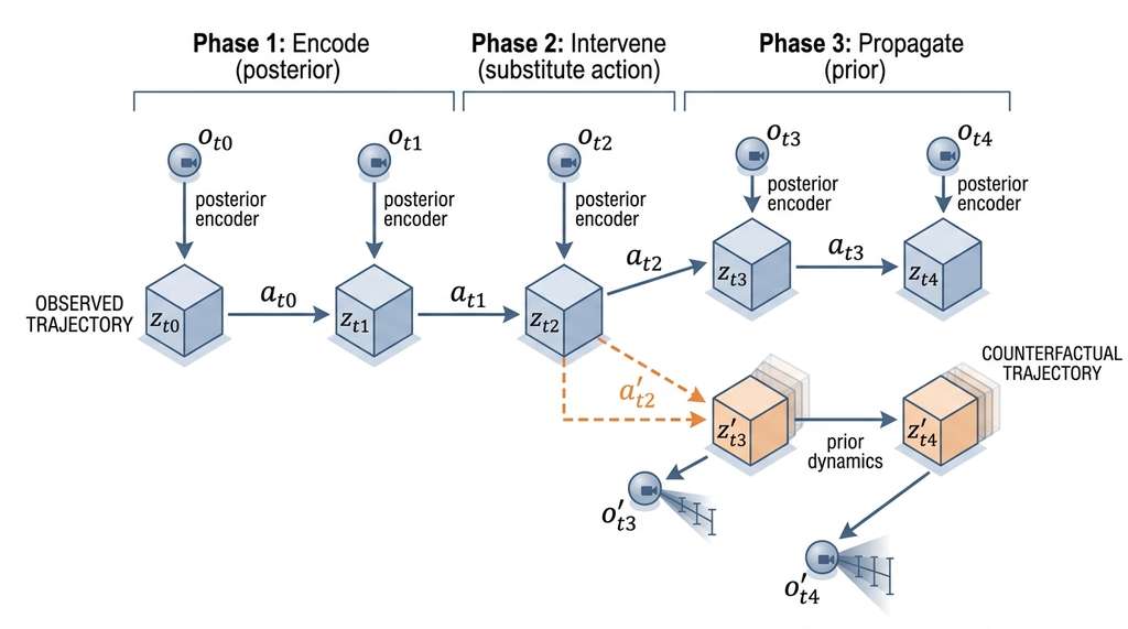
forward again. Figure 44.3 below illustrates this branching structure, showing
how the factual and counterfactual trajectories share a common encoded history up to
the intervention point and then diverge.
Counterfactual reasoning asks: "what would the outcome have been
if a specific variable had taken a different value, while everything else remained
the same?" This question matters because it is the only way to evaluate
interventions that no one actually tried, the core task of experimental
science and evidence-based decision making. The mechanism
encodes the observed history into a latent state, preserving all context up to the
intervention point. It then substitutes the hypothetical action and propagates
dynamics forward under the learned model to produce the alternative trajectory.
Use counterfactual
analysis rather than simple what-if simulation when you need to reason about a
specific observed case rather than a generic starting condition. For
generic exploration of action effects from arbitrary states, standard forward rollouts
(the imagine() method from Section 44.1) are sufficient and cheaper.
This practical distinction rests on a formal theoretical hierarchy that clarifies exactly what each type of reasoning can and cannot do.
Pearl (2009) formalized three levels of causal reasoning, each strictly more powerful than the last:
- Association (seeing): \(P(Y | X)\). "Patients who take the drug have lower blood pressure." This is correlation, observable from passive data.
- Intervention (doing): \(P(Y | \text{do}(X))\), where the do-operator \(\text{do}(X)\) denotes forcibly setting a variable to a value rather than passively observing it. "If we administer the drug, blood pressure will decrease." This requires a causal model that distinguishes action from observation.
- Counterfactual (imagining): \(P(Y_{X=x'} | X=x, Y=y)\). "Given that this specific patient took the drug and their blood pressure dropped, what would have happened if they had not taken it?" This requires a structural model of the individual case.
A standard neural network trained on observational data operates at Level 1: it
captures correlations but cannot distinguish causation from confounding. A world
model trained on interventional data (trajectories where actions are applied to the
environment) operates at Level 2: its imagine() method implements the
do-operator by replacing the action in the dynamics and rolling forward. With
additional machinery, we can push it to Level 3: counterfactual reasoning about
specific observed trajectories.
The critical ingredient for counterfactual reasoning is the RSSM's posterior encoder. Given an observed trajectory, the posterior maps each observation into a latent state \(z_t = (h_t, s_t)\) that captures all the specific details of that particular trajectory (the actual temperature, the actual catalyst concentration, the actual mixing rate). To ask "what if?", we rewind to a specific time step \(t_0\), keep the posterior state \(z_{t_0}\) (which encodes the actual conditions at that moment), substitute a different action \(a'_{t_0}\), and then roll forward using the prior (since we no longer have real observations for the counterfactual future). The posterior anchors us to the specific case; the prior propagates the consequences of the intervention.
Mental Model
Think of counterfactual reasoning like replaying a chess game from a recorded transcript. You follow the exact moves both players made up to move 14 (encoding the observed trajectory through the posterior). Then you ask: "What if White had moved the bishop instead of the knight on move 14?" You keep the entire board position as it actually was at move 14 (the posterior state), substitute the bishop move (the counterfactual action), and then play out the rest of the game using your best judgment about how both players would respond (the prior). The board position at move 14 anchors you to the specific game that was played; your judgment about subsequent moves is your learned model of chess dynamics. The further you play past move 14, the less confident you should be, because each subsequent move compounds your uncertainty about what would have happened.
2. Implementing Counterfactual Rollouts
The counterfactual procedure has three steps: (1) encode the observed trajectory through the posterior to recover latent states, (2) select an intervention point and substitute a different action, (3) roll forward from the intervention point using the prior. Let us implement this. In short: the posterior anchors the counterfactual to a real history; the prior propagates the road not taken. Figure 44.2.1 illustrates counterfactual rollout procedure with posterior encoding and prior propagation.
import torch
import numpy as np
from typing import Optional


class CounterfactualAnalyzer:
    """Counterfactual reasoning engine using a trained RSSM.

    Given an observed trajectory and a hypothetical intervention,
    produces counterfactual predictions with confidence estimates.
    """

    def __init__(self, rssm, n_samples: int = 50):
        """
        Args:
            rssm: trained RSSM model (from Listing 44.1)
            n_samples: number of stochastic samples for confidence intervals
        """
        self.rssm = rssm
        self.n_samples = n_samples
        self.rssm.eval()

    @torch.no_grad()
    def encode_trajectory(self, observations, actions):
        """Encode an observed trajectory through the posterior.

        Args:
            observations: (1, T, obs_dim) observed trajectory
            actions: (1, T, act_dim) actions taken

        Returns:
            Lists of deterministic states h_t and stochastic states s_t.
        """
        device = next(self.rssm.parameters()).device
        obs = observations.to(device)
        act = actions.to(device)

        h, s = self.rssm.initial_state(1, device)
        h_states = [h]
        s_states = [s]

        T = obs.shape[1]
        for t in range(T):
            h = self.rssm.sequence_step(h, s, act[:, t])
            s, _, _ = self.rssm.posterior(h, obs[:, t])
            h_states.append(h)
            s_states.append(s)

        return h_states, s_states

    @torch.no_grad()
    def counterfactual_rollout(
        self,
        observations: torch.Tensor,
        actions: torch.Tensor,
        intervention_step: int,
        counterfactual_actions: torch.Tensor,
        horizon: Optional[int] = None,
    ):
        """Compute counterfactual predictions.

        Args:
            observations: (1, T, obs_dim) the observed trajectory
            actions: (1, T, act_dim) the original actions
            intervention_step: time step at which to intervene
            counterfactual_actions: (1, H, act_dim) alternative actions
                starting at intervention_step
            horizon: how many steps to roll out (default: len of
                counterfactual_actions)

        Returns:
            Dictionary with factual predictions, counterfactual
            predictions, and confidence intervals.
        """
        if horizon is None:
            horizon = counterfactual_actions.shape[1]

        device = next(self.rssm.parameters()).device
        counterfactual_actions = counterfactual_actions.to(device)

        # Step 1: encode the observed trajectory
        h_states, s_states = self.encode_trajectory(observations, actions)

        # Step 2: get the latent state at the intervention point
        # (index is intervention_step because h_states[0] is initial)
        h_intervene = h_states[intervention_step]
        s_intervene = s_states[intervention_step]

        # Step 3: factual rollout (continue with original actions)
        factual_obs = []
        factual_rewards = []
        h, s = h_intervene.clone(), s_intervene.clone()
        for t in range(horizon):
            act_idx = intervention_step + t
            if act_idx < actions.shape[1]:
                a = actions[:, act_idx].to(device)
            else:
                a = torch.zeros(1, actions.shape[-1], device=device)
            h = self.rssm.sequence_step(h, s, a)
            s, _, _ = self.rssm.prior(h)
            obs_pred, rew_pred = self.rssm.decode(h, s)
            factual_obs.append(obs_pred)
            factual_rewards.append(rew_pred)

        # Step 4: counterfactual rollout with multiple samples
        cf_obs_samples = []
        cf_rew_samples = []

        for _ in range(self.n_samples):
            h, s = h_intervene.clone(), s_intervene.clone()
            sample_obs = []
            sample_rew = []
            for t in range(horizon):
                a = counterfactual_actions[:, t]
                h = self.rssm.sequence_step(h, s, a)
                s, _, _ = self.rssm.prior(h)
                obs_pred, rew_pred = self.rssm.decode(h, s)
                sample_obs.append(obs_pred)
                sample_rew.append(rew_pred)
            cf_obs_samples.append(torch.stack(sample_obs, dim=1))
            cf_rew_samples.append(torch.stack(sample_rew, dim=1))

        # Aggregate counterfactual samples
        cf_obs_all = torch.stack(cf_obs_samples, dim=0)  # (n_samples, 1, H, obs)
        cf_rew_all = torch.stack(cf_rew_samples, dim=0)

        return {
            "factual_obs": torch.stack(factual_obs, dim=1),
            "factual_rewards": torch.stack(factual_rewards, dim=1),
            "counterfactual_obs_mean": cf_obs_all.mean(dim=0),
            "counterfactual_obs_std": cf_obs_all.std(dim=0),
            "counterfactual_rewards_mean": cf_rew_all.mean(dim=0),
            "counterfactual_rewards_std": cf_rew_all.std(dim=0),
            "counterfactual_obs_samples": cf_obs_all,
            "intervention_step": intervention_step,
            "horizon": horizon,
}The distinction between the factual and counterfactual branches is subtle but important. Both start from the same latent state \(z_{t_0}\), which encodes the actual conditions at the intervention point. The factual branch continues with the original actions; the counterfactual branch substitutes different actions. Both use the prior for forward prediction because we want a fair comparison: the factual branch should not have an unfair advantage from seeing the actual observations.
Common Misconception
A frequent mistake is believing that a counterfactual rollout is the same as simply re-running a simulation from different initial conditions. It is not. A counterfactual preserves the exact observed state at the intervention point (encoded by the posterior from real data), then changes only the action while keeping all latent context intact. Re-running from different initial conditions discards the specific history that led to the current state, and therefore answers a fundamentally different question: "what happens from state X?" rather than "what would have happened to this particular trajectory if the action had been different?"
A clinical researcher observes a patient's 10-day treatment trajectory: daily blood pressure readings (observations), drug doses (actions), and symptom scores (rewards). On day 3, the clinician increased the dose from 10mg to 20mg. The patient's blood pressure dropped sharply on days 4-5 but rebounded on days 6-7. The counterfactual question: "What would have happened if we had increased to only 15mg on day 3?" The analyzer encodes the full 10-day observed trajectory, rewinds to day 3, substitutes the 15mg action, and rolls forward. The counterfactual prediction (with confidence intervals from 50 stochastic samples) suggests that the 15mg dose would have produced a slower but more sustained blood pressure reduction, without the rebound. This counterfactual insight, which cannot be obtained from the observational data alone, guides the design of future dosing protocols.
3. Confidence Calibration for Counterfactuals
The counterfactual rollouts of the previous section produced predictions with multiple stochastic samples, but the drug dosing example already raised the crucial follow-up: how much should we trust those predictions?
Counterfactual predictions grow less reliable as the hypothetical action diverges from the observed action and as the rollout horizon lengthens. A responsible analysis system must quantify this uncertainty and flag untrustworthy predictions.
We use three complementary measures of counterfactual confidence:
Three Signals of Counterfactual Reliability
Stochastic spread. The standard deviation across multiple stochastic samples from the prior captures aleatoric uncertainty, where aleatoric uncertainty is the irreducible randomness inherent in the system's dynamics (as opposed to epistemic uncertainty, which shrinks with more data). Wide spread means the outcome is highly sensitive to stochastic factors that the model cannot predict deterministically.
Action distance. The distance between the counterfactual action and the observed action, \(\| a'_t - a_t \|\), serves as a proxy for how far we are extrapolating from the training distribution. World models tend to be more reliable when interpolating within the training distribution than when extrapolating beyond it; large action distances warrant skepticism.
Horizon decay. Prediction error compounds over time (we quantify this precisely in Section 44.3). A counterfactual prediction at horizon \(H\) carries roughly \(\sqrt{H}\) times the single-step uncertainty under independent-error assumptions (as implemented in Listing 44.6), though nonlinear error interactions can push the actual growth rate higher. We apply an exponential discount to confidence as the horizon grows.
Checkpoint
So far: counterfactual confidence rests on three independent signals: stochastic spread (how much the model's own samples disagree), action distance (how far the hypothetical action is from what was actually done), and horizon decay (how far into the future we are predicting), and Listing 44.6 below combines them multiplicatively into a single per-step score.
def compute_counterfactual_confidence(
    cf_result: dict,
    original_actions: torch.Tensor,
    counterfactual_actions: torch.Tensor,
    single_step_rmse: float,
    decay_rate: float = 0.15,
) -> dict:
    """Compute confidence scores for counterfactual predictions.

    Args:
        cf_result: output from CounterfactualAnalyzer.counterfactual_rollout
        original_actions: (1, T, act_dim) original action sequence
        counterfactual_actions: (1, H, act_dim) alternative actions
        single_step_rmse: one-step prediction root mean square error (RMSE)
            (from validation)
        decay_rate: exponential decay rate for horizon confidence

    Returns:
        Dictionary with per-step confidence scores and overall rating.
    """
    horizon = cf_result["horizon"]
    t0 = cf_result["intervention_step"]

    # 1. Stochastic spread (normalized by observation magnitude)
    obs_std = cf_result["counterfactual_obs_std"].squeeze(0)  # (H, obs_dim)
    obs_mean = cf_result["counterfactual_obs_mean"].squeeze(0).abs() + 1e-6
    normalized_spread = (obs_std / obs_mean).mean(dim=-1)  # (H,)

    # 2. Action distance at each step
    orig_slice = original_actions[
        :, t0:t0 + horizon
    ].squeeze(0)  # (H, act_dim)
    cf_slice = counterfactual_actions.squeeze(0)[:horizon]
    action_dist = torch.norm(
        cf_slice - orig_slice, dim=-1
    )  # (H,)
    max_action_dist = action_dist.max() + 1e-6
    normalized_action_dist = action_dist / max_action_dist

    # 3. Horizon decay
    steps = torch.arange(horizon, dtype=torch.float32)
    horizon_confidence = torch.exp(-decay_rate * steps)

    # Compound error estimate: RMSE grows roughly as sqrt(H)
    error_estimate = single_step_rmse * torch.sqrt(steps + 1)

    # Combined confidence: product of three factors
    spread_confidence = torch.exp(-2.0 * normalized_spread)
    action_confidence = torch.exp(-1.0 * normalized_action_dist)
    per_step_confidence = (
        spread_confidence * action_confidence * horizon_confidence
    )

    # Overall confidence: geometric mean across steps
    overall_confidence = per_step_confidence.prod().pow(1.0 / horizon).item()

    # Qualitative rating
    if overall_confidence > 0.7:
        rating = "HIGH"
    elif overall_confidence > 0.4:
        rating = "MODERATE"
    elif overall_confidence > 0.2:
        rating = "LOW"
    else:
        rating = "UNRELIABLE"

    return {
        "per_step_confidence": per_step_confidence.numpy(),
        "overall_confidence": overall_confidence,
        "rating": rating,
        "error_estimate_per_step": error_estimate.numpy(),
        "stochastic_spread": normalized_spread.numpy(),
        "action_distance": normalized_action_dist.numpy(),
}A subtle but critical point: counterfactual predictions are less reliable than ordinary predictions at the same horizon, even when both use the same world model. The reason is distributional shift (a mismatch between the states the model encounters during counterfactual rollout and the states it was trained on). Ordinary predictions extrapolate the current trajectory forward; the model has been trained on similar trajectories. A counterfactual applies an action the model may never have seen from this particular state. The further the counterfactual action departs from the behavioral policy (the policy that generated the training data)'s distribution, the more the model must extrapolate, and the less trustworthy its predictions become. This is why the action distance term in the confidence score is essential.
4. Causal Structure Discovery Through Interventions
Beyond answering individual "what-if" questions, systematic counterfactual analysis reveals the causal structure of the environment. By intervening on each action dimension independently and measuring the effect on each observation dimension, we can construct a causal influence matrix that shows which actions affect which outcomes.
def discover_causal_structure(
    analyzer: "CounterfactualAnalyzer",
    observations: torch.Tensor,
    actions: torch.Tensor,
    intervention_step: int,
    perturbation_scale: float = 0.5,
    horizon: int = 5,
) -> np.ndarray:
    """Discover causal structure by systematic intervention.

    For each action dimension, perturb it independently and measure
    the effect on each observation dimension. The resulting matrix
    reveals which actions causally influence which observations.

    Args:
        analyzer: trained CounterfactualAnalyzer
        observations: (1, T, obs_dim) reference trajectory
        actions: (1, T, act_dim) reference actions
        intervention_step: when to intervene
        perturbation_scale: magnitude of perturbation
        horizon: rollout length after intervention

    Returns:
        Causal influence matrix (act_dim, obs_dim) where entry (i, j)
        measures how much action dimension i affects observation dim j.
    """
    act_dim = actions.shape[-1]
    obs_dim = observations.shape[-1]
    influence_matrix = np.zeros((act_dim, obs_dim))

    # Baseline: counterfactual with original actions (should match factual)
    cf_actions_base = actions[:, intervention_step:intervention_step + horizon]

    for act_idx in range(act_dim):
        # Perturb only action dimension act_idx
        cf_actions_plus = cf_actions_base.clone()
        cf_actions_plus[:, 0, act_idx] += perturbation_scale

        cf_actions_minus = cf_actions_base.clone()
        cf_actions_minus[:, 0, act_idx] -= perturbation_scale

        # Run counterfactual rollouts
        result_plus = analyzer.counterfactual_rollout(
            observations, actions, intervention_step,
            cf_actions_plus, horizon
        )
        result_minus = analyzer.counterfactual_rollout(
            observations, actions, intervention_step,
            cf_actions_minus, horizon
        )

        # Measure effect: difference in predicted observations
        delta_obs = (
            result_plus["counterfactual_obs_mean"]
            - result_minus["counterfactual_obs_mean"]
        )
        # Average absolute effect over horizon
        influence = delta_obs.abs().mean(dim=1).squeeze(0).numpy()
        influence_matrix[act_idx] = influence

    # Normalize each row to [0, 1]
    row_maxes = influence_matrix.max(axis=1, keepdims=True)
    row_maxes[row_maxes == 0] = 1.0
    influence_matrix = influence_matrix / row_maxes

return influence_matrixThis perturbation-based approach connects directly to the causal discovery methods of Chapter 31. The influence matrix approximates the Jacobian (the matrix of partial derivatives \(\partial f_j / \partial x_i\), measuring how each output dimension responds to an infinitesimal change in each input dimension) of the causal mechanism: \(\frac{\partial \mathbb{E}[o_{t+1}]}{\partial \text{do}(a_t)}\). Unlike the purely observational methods of Chapter 31 (PC algorithm, NOTEARS), this approach uses interventional data by construction: the world model trained on trajectories where actions were applied. It can therefore distinguish genuine causal effects from spurious correlations due to confounders.
A bioprocess engineer controls a bioreactor with five action dimensions: feed rate,
temperature setpoint, pH setpoint, dissolved oxygen target, and agitation speed.
The observations include cell density, product concentration, nutrient levels, and
waste metabolite concentration. Running discover_causal_structure()
reveals that feed rate strongly influences cell density and nutrient levels (as
expected) but that dissolved oxygen has an unexpectedly strong influence on product
concentration (potentially through a metabolic switch). The temperature setpoint
shows a strong delayed effect on waste metabolite concentration but minimal effect
on cell density at the current operating point. These causal insights, extracted
automatically from the world model, suggest that optimizing product yield should
focus on dissolved oxygen control rather than the traditionally emphasized
temperature profile.
Research Frontier
TD-MPC2 (Hansen et al., 2024, "TD-MPC2: Scalable, Robust World Models for Continuous Control," ICLR 2024) demonstrated that a single world model architecture, trained once across 104 continuous control tasks spanning multiple domains, can support both planning and counterfactual reasoning without per-task fine-tuning. Its implicit latent dynamics (learned via temporal difference objectives rather than explicit reconstruction) may produce tighter counterfactual confidence bounds than reconstruction-based models like the RSSM, because the latent space is optimized directly for action-conditional prediction rather than observation fidelity. This suggests that the next generation of counterfactual analysis tools may not need the explicit posterior/prior separation described in this section; instead, a single learned value-aware dynamics model can serve both forward planning and backward counterfactual queries, with calibration emerging from the TD loss itself.
5. Counterfactual Explanation of Anomalies
Causal structure discovery tells us which actions influence which outcomes in general; the natural next step is using counterfactual reasoning to diagnose why a specific outcome went wrong.
One powerful application of counterfactual reasoning is explaining anomalies detected by the methods of Chapter 30. When an observation deviates from the world model's prediction (a large reconstruction error or a high Kullback-Leibler (KL) divergence between prior and posterior), we can ask: "What action would have been needed to prevent this anomaly?" The answer identifies the controllable cause of the anomalous event.
def explain_anomaly(
    analyzer: "CounterfactualAnalyzer",
    observations: torch.Tensor,
    actions: torch.Tensor,
    anomaly_step: int,
    target_obs: torch.Tensor,
    n_optimization_steps: int = 100,
    lr: float = 0.01,
) -> dict:
    """Find the counterfactual action that would have prevented an anomaly.

    Uses gradient-based optimization to find the action at anomaly_step-1
    that would have produced the target (normal) observation at anomaly_step.

    Args:
        analyzer: trained CounterfactualAnalyzer
        observations: (1, T, obs_dim) trajectory containing the anomaly
        actions: (1, T, act_dim) original actions
        anomaly_step: the time step where the anomaly occurred
        target_obs: (obs_dim,) the "normal" observation we wish we had seen
        n_optimization_steps: gradient descent iterations
        lr: learning rate for action optimization

    Returns:
        Dictionary with optimal counterfactual action and explanation.
    """
    rssm = analyzer.rssm
    device = next(rssm.parameters()).device

    # Encode trajectory up to anomaly
    h_states, s_states = analyzer.encode_trajectory(observations, actions)

    # Get state just before the anomaly
    h_pre = h_states[anomaly_step - 1].detach()
    s_pre = s_states[anomaly_step - 1].detach()

    # Initialize counterfactual action from the original
    original_action = actions[:, anomaly_step - 1].to(device).detach()
    cf_action = original_action.clone().requires_grad_(True)
    target = target_obs.to(device)

    optimizer = torch.optim.Adam([cf_action], lr=lr)
    best_action = cf_action.clone().detach()
    best_loss = float("inf")

    # Enable gradients temporarily for optimization
    rssm.train()
    for step in range(n_optimization_steps):
        optimizer.zero_grad()
        h = rssm.sequence_step(h_pre, s_pre, cf_action)
        s, _, _ = rssm.prior(h)
        obs_pred, _ = rssm.decode(h, s)

        loss = torch.nn.functional.mse_loss(obs_pred.squeeze(), target)

        # Regularize: prefer small deviations from original action
        action_reg = 0.1 * torch.norm(cf_action - original_action)
        total_loss = loss + action_reg

        total_loss.backward()
        optimizer.step()

        if total_loss.item() < best_loss:
            best_loss = total_loss.item()
            best_action = cf_action.clone().detach()

    rssm.eval()

    action_delta = (best_action - original_action).squeeze()

    return {
        "original_action": original_action.squeeze().cpu().numpy(),
        "counterfactual_action": best_action.squeeze().cpu().numpy(),
        "action_delta": action_delta.cpu().numpy(),
        "reconstruction_loss": best_loss,
        "explanation": _format_explanation(action_delta.cpu().numpy()),
    }


def _format_explanation(delta: np.ndarray, threshold: float = 0.05) -> str:
    """Generate human-readable explanation from action delta."""
    significant = np.where(np.abs(delta) > threshold)[0]
    if len(significant) == 0:
        return (
            "The anomaly cannot be explained by action changes alone. "
            "It may be due to unobserved external factors."
        )
    parts = []
    for idx in significant:
        direction = "increasing" if delta[idx] > 0 else "decreasing"
        parts.append(
            f"action dimension {idx} by {abs(delta[idx]):.3f} ({direction})"
        )
return "The anomaly could have been prevented by changing: " + "; ".join(parts)The counterfactual action that "would have prevented" an anomaly is not necessarily the root cause of the anomaly. It is the controllable lever that, if moved, would have changed the outcome. The actual root cause may be an unobserved disturbance (equipment malfunction, contamination, external perturbation) that the world model cannot represent because it was not in the training data. Always present counterfactual explanations as "the action change that would have compensated for the anomaly," not as "the cause of the anomaly." This distinction matters for scientific integrity and for the responsible discovery practices discussed in Chapter 57.
6. Batch Counterfactual Analysis for Experiment Design
The single-trajectory counterfactual analysis above answers one question at a time. For experiment design (Chapter 46), we often want to explore an entire space of counterfactual actions to identify the most informative experiment to run next. This connects counterfactual reasoning to active learning: the best next experiment is the one whose counterfactual prediction has the highest uncertainty (because that is where the world model needs the most data).
def counterfactual_experiment_candidates(
    analyzer: "CounterfactualAnalyzer",
    observations: torch.Tensor,
    actions: torch.Tensor,
    intervention_step: int,
    candidate_actions: torch.Tensor,
    horizon: int = 5,
) -> dict:
    """Rank candidate experiments by counterfactual informativeness.

    For each candidate action, computes the counterfactual prediction
    and its uncertainty. Actions that produce high-uncertainty
    counterfactual predictions are the most informative to test.

    Args:
        analyzer: trained CounterfactualAnalyzer
        observations: (1, T, obs_dim) reference trajectory
        actions: (1, T, act_dim) reference actions
        intervention_step: when to intervene
        candidate_actions: (N, H, act_dim) candidate action sequences
        horizon: rollout horizon

    Returns:
        Dictionary with ranked candidates, uncertainties, and predictions.
    """
    n_candidates = candidate_actions.shape[0]
    uncertainties = []
    predictions = []

    for i in range(n_candidates):
        cf_actions = candidate_actions[i:i+1]
        result = analyzer.counterfactual_rollout(
            observations, actions, intervention_step,
            cf_actions, horizon
        )
        # Uncertainty: mean std across observation dims and horizon
        uncertainty = result["counterfactual_obs_std"].mean().item()
        prediction = result["counterfactual_rewards_mean"].sum().item()
        uncertainties.append(uncertainty)
        predictions.append(prediction)

    uncertainties = np.array(uncertainties)
    predictions = np.array(predictions)

    # Rank by uncertainty (most informative first)
    info_ranking = np.argsort(-uncertainties)
    # Rank by predicted reward (most promising first)
    reward_ranking = np.argsort(-predictions)

    return {
        "uncertainties": uncertainties,
        "predicted_rewards": predictions,
        "informativeness_ranking": info_ranking,
        "reward_ranking": reward_ranking,
        "most_informative_idx": info_ranking[0],
        "most_promising_idx": reward_ranking[0],
}For counterfactual reasoning on tabular (non-sequential) data, the DoWhy library provides a complete causal inference pipeline including counterfactual estimation. What required 200+ lines of custom code above (for the sequential RSSM-based case) is a five-line call for the tabular case:
import dowhy

model = dowhy.CausalModel(data=df, treatment="temperature",
                          outcome="yield", graph=causal_graph)
identified = model.identify_effect()
estimate = model.estimate_effect(identified, method_name="backdoor.linear_regression")
counterfactual = model.do(x={"temperature": 350}) # do(T=350)CausalModel wraps a causal graph and dataset, identify_effect() selects an estimand, and do() computes the interventional distribution for a specified treatment value.
DoWhy handles confounding adjustment, sensitivity analysis, and refutation tests
internally. As of 2024, DoWhy is part of the broader PyWhy ecosystem and offers a newer
Graphical Causal Model (GCM) API alongside the classic CausalModel interface
shown above; the GCM API supports more flexible counterfactual estimation, including
intrinsic causal influence and distributional counterfactuals. Use it when your data is tabular and your causal graph is known; use the
RSSM-based approach when you have sequential decision data and need multi-step
counterfactual rollouts.
7. Integrating Counterfactuals into the Discovery Workbench
In the Discovery Workbench, the CounterfactualAnalyzer extends the world
model backend introduced in Section 44.1. When a scientist observes an unexpected
experimental result, the Workbench offers three analysis modes:
- What-if analysis: the scientist specifies an alternative action and the Workbench shows the counterfactual trajectory with confidence intervals.
- Anomaly explanation: the Workbench automatically identifies the minimal action change that would have produced the expected result, using the gradient-based optimization from Listing 44.8.
- Next experiment recommendation: the Workbench evaluates a grid of candidate actions using Listing 44.9 and recommends the most informative or most promising experiment to run next.
All three modes feed their results back into the Workbench's experiment registry (Chapter 47), creating a full audit trail of real experiments, counterfactual analyses, and the reasoning that led to each experimental decision.
Try It: Counterfactual Temperature Sweep on a Toy Chemical Reactor
Build a minimal counterfactual analysis pipeline using only NumPy and Matplotlib (no GPU required). The steps:
- Simulate a toy exothermic reactor using the ODE ordinary differential equation (ODE) \(\frac{dC}{dt} = -k_0 e^{-E_a / T} C\) (first-order Arrhenius kinetics). Generate 50 trajectories with random temperature profiles \(T(t)\) drawn uniformly from [300K, 400K] over 100 time steps, recording concentration \(C(t)\) as the observation and \(T(t)\) as the action.
- Train a small multi-layer perceptron (MLP) dynamics model: given \((C_t, T_t)\), predict \(C_{t+1}\). Split
your 50 trajectories into 40 for training and 10 for validation. Use
torch.nn.Linearwith two hidden layers of 64 units and ReLU activations. Train for 200 epochs with Adam (lr=1e-3). - Pick one validation trajectory. Encode it by feeding the real observations through the model step by step. At step 30, substitute a range of counterfactual temperatures: 310K, 330K, 350K, 370K, 390K. Roll each forward for 50 steps using the trained model.
- For each counterfactual temperature, run the true ODE with that temperature from the same \(C_{30}\) to get ground-truth counterfactual trajectories. Compare the model's counterfactual predictions to the ODE ground truth.
- Plot all five counterfactual trajectories (model prediction vs. ground truth) on one figure with Matplotlib. Add shading for the model's prediction error. Observe how prediction error grows with both horizon length and deviation from the training distribution's mean temperature.
Exercise 44.2.1
Suppose you have a trained world model for a two-variable system (temperature \(T\) and
pressure \(P\)) and an observed trajectory of 20 time steps. You intervene at step 10,
changing the temperature action from 350K to 400K. After rolling out the counterfactual
for 10 steps, you obtain a stochastic spread (normalized standard deviation) of 0.8 at
step 5 of the rollout. Using the confidence formula from Listing 44.6 with
decay_rate=0.15, and assuming the action distance term contributes
exp(-1.0 * 0.3) = 0.741, compute the per-step confidence at rollout
step 5. Is this prediction trustworthy enough to guide a real experiment?
Hint
The three multiplicative factors are: spread confidence = exp(-2.0 * 0.8),
action confidence = 0.741, and horizon confidence = exp(-0.15 * 5).
Multiply all three. Compare the result to the qualitative thresholds: above 0.7 is HIGH,
above 0.4 is MODERATE, above 0.2 is LOW, below 0.2 is UNRELIABLE.
Step-Through: Counterfactual Rollout on a 3-Step Trajectory
Trace the counterfactual_rollout procedure with concrete numbers. Suppose
our RSSM has 2-dimensional latent states and 1-dimensional observations and actions.
- Observed trajectory: observations = [1.0, 1.5, 2.3], actions = [0.2, 0.4, 0.6].
- Encode via posterior: feeding each (obs, action) pair yields posterior states \(z_0 = (h_0, s_0)\), \(z_1 = (h_1, s_1) = ([0.3, 0.7], [0.1, 0.4])\), \(z_2 = (h_2, s_2)\), \(z_3 = (h_3, s_3)\).
- Intervention at step 1: we keep \(z_1 = ([0.3, 0.7], [0.1, 0.4])\) and substitute action \(a'_1 = 0.9\) instead of \(a_1 = 0.4\).
- Prior rollout step 1: \(h'_2 = \text{GRU}([0.3, 0.7], [0.1, 0.4], 0.9) = [0.5, 0.2]\) (the Gated Recurrent Unit (GRU) now processes the counterfactual action). Sample \(s'_2 \sim \text{prior}(h'_2) = [0.3, 0.1]\).
- Decode: \(\hat{o}'_2 = \text{decode}([0.5, 0.2], [0.3, 0.1]) = 2.8\). Compare to the factual \(\hat{o}_2 = 2.3\). The higher counterfactual action (0.9 vs. 0.4) produced a higher predicted observation (2.8 vs. 2.3).
- Repeat for the next step using \(h'_2, s'_2\) and the next counterfactual action. Each step compounds uncertainty because \(s'\) is sampled from the prior (no real observation to anchor it).
Real-World Application: DeepMind's Counterfactual Policy Evaluation in Data Centers
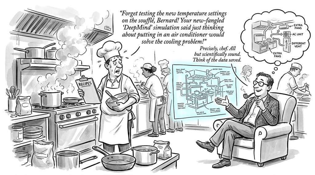
Google DeepMind applied counterfactual reasoning with learned world models to evaluate alternative cooling strategies in production data centers without physically testing them. The system encodes the observed thermal trajectory of a data center hall (server loads, ambient temperature, coolant flow rates) into a latent state, then asks: "What would the Power Usage Effectiveness (PUE) have been if we had raised the chilled water setpoint by 2 degrees Fahrenheit?" By running thousands of such counterfactual queries against historical operating data, the team identified safe energy-saving interventions that reduced cooling energy by roughly 40% (circa 2016), all before committing to any physical change.
The Grandmother of All Counterfactuals
The philosophical roots of counterfactual reasoning predate AI by centuries. In 1748, David Hume argued that our very notion of causation is built on counterfactual thinking: we say fire causes heat because we believe that if the fire had not been lit, the room would have remained cold. Pearl's do-calculus, which underlies the machinery in this section, finally gave Hume's intuition a rigorous mathematical foundation 250 years later. The irony: it took a computer scientist to formalize what an 18th-century philosopher articulated over afternoon tea.
Lab: Counterfactual Sensitivity Map for CartPole
Goal: build a visual "sensitivity map" showing how counterfactual outcomes change as you vary both the intervention time and the magnitude of the alternative action in the CartPole environment.
Tools needed: Python 3.8+, PyTorch, Gymnasium (pip install gymnasium),
Matplotlib, and the RSSM implementation from Section 44.1 (or a simple 2-layer MLP
dynamics model as a stand-in).
Procedure (20 minutes): (1) Collect 200 CartPole episodes using a random policy and train a dynamics model on them. (2) Select one episode where the pole falls at step ~40. (3) For each intervention time \(t_0 \in \{5, 10, 15, 20, 25, 30, 35\}\) and each counterfactual force \(a' \in \{-1.0, -0.5, 0.0, 0.5, 1.0\}\), run a counterfactual rollout of 20 steps and record the predicted pole angle at the final step. (4) Plot the results as a heatmap (x-axis: intervention time, y-axis: counterfactual force, color: final pole angle).
What to vary: try different episodes (ones that fail early vs. late) and different training set sizes (50 vs. 200 episodes). What to observe: the heatmap should show a "corridor of controllability" where early interventions with moderate forces keep the pole upright, while late interventions require extreme forces and produce high-uncertainty predictions (visible as noisy regions in the map).
Exercises
-
(Conceptual) Explain the difference between Pearl's three levels of
causal reasoning (association, intervention, counterfactual). At which level does
the RSSM's
imagine()method operate? At which level does theCounterfactualAnalyzeroperate? Justify your answers. -
(Coding) Implement a counterfactual analysis of a CartPole trajectory.
Train an RSSM on CartPole trajectories (using the code from Section 44.1), then
use the
CounterfactualAnalyzerto answer: "At the moment the pole started falling, what force should I have applied to keep it balanced?" Visualize both the factual and counterfactual trajectories. -
(Analysis) Run
discover_causal_structure()on a trained RSSM for the Pendulum environment. Compare the discovered causal influence matrix to the known physics of the pendulum (torque affects angular velocity, which affects angle). Does the world model recover the correct causal structure? - (Research) The confidence scoring in Listing 44.6 uses three heuristic factors. Design and implement a calibration experiment: generate 1000 counterfactual predictions with known ground truth (by running the actual environment), then check whether the confidence scores are well-calibrated (i.e., 70% confidence predictions are correct 70% of the time). If not, propose and implement a recalibration method.
What's Next
We have used world models to reason about what happened and what might have happened. In Section 44.3: Building a World Model Planner, we turn to the forward-looking question: what should we do? We build a complete model-based planner that selects actions by imagining thousands of future trajectories, and we confront the fundamental challenge of compound error accumulation over long planning horizons.
Bibliography
The foundational text on causal inference, defining the three-level causal hierarchy (association, intervention, counterfactual) that structures this section.
DreamerV3, whose RSSM architecture provides the posterior encoding and prior rollout mechanisms we use for counterfactual reasoning.
The DoWhy library for causal inference on tabular data, providing a complementary approach to the sequential RSSM-based counterfactual analysis.
Empirical evaluation of causal discovery methods applied to learned world models, showing when perturbation-based approaches succeed and fail.
Using counterfactual reasoning in model-based RL to improve policy learning from off-policy data.