44.3 Building a World Model Planner

1. Model Predictive Control with Learned Dynamics

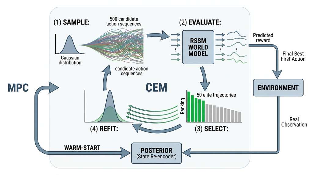
A robot chemist stares at a half-finished reaction, 500 possible next moves flickering through its learned simulator in under a second, yet it commits to just one, watches what actually happens, and immediately replans from scratch. That loop is Model Predictive Control (MPC), a planning framework with a simple structure: at each time step, solve an optimization problem to find the best action sequence over a future horizon \(H\), execute only the first action, observe the real next state, and re-plan. The re-planning step is critical: it corrects for prediction errors by grounding the planner in the actual state after each step. The MPC loop is illustrated in Figure 44.5.

Formally, at time \(t\) with current state \(z_t = (h_t, s_t)\), MPC solves:

where \(\hat{r}\) is the world model's reward predictor, \(\gamma\) is a discount factor, and the RSSM's imagine() method supplies the dynamics \(z_{t+k+1} = f_\text{wm}(z_{t+k}, a_{t+k})\). After solving, the agent executes only \(a^*_t\) in the real environment and observes the next real state. It then re-encodes that state through the posterior and re-plans from scratch. This "plan, execute one step, re-plan" loop is the heartbeat of MPC.

The re-planning loop explains when to act, but it leaves open the question of how to choose the best action sequence at each step.

2. The Cross-Entropy Method (CEM) for Action Optimization

Without a reliable optimizer for this planning step, a world model planner defaults to random search, which scales so poorly that useful plans become impossible in action spaces with more than a handful of dimensions. The Cross-Entropy Method solves this bottleneck.

The optimization problem in MPC is typically non-convex and cannot be solved in closed form. We need a derivative-free optimizer (an optimization algorithm that does not require computing gradients of the objective function) that can handle the world model as a black box (even though the model is differentiable, CEM is often more robust in practice). The Cross-Entropy Method works by iteratively sampling action sequences from a distribution, evaluating them in the world model, and refitting the distribution to the top-performing samples.

The Cross-Entropy Method is a population-based optimization algorithm that maintains a probability distribution (typically a diagonal Gaussian, where each dimension is an independent Gaussian with its own mean and variance) over the solution space and iteratively narrows it toward high-performing regions. It matters because it provides a simple, parallelizable way to solve the non-convex planning problem without requiring gradient computation, making it compatible with any black-box simulator or learned model. The mechanism works in three repeated steps: sample a large batch of candidate solutions from the current distribution, evaluate all candidates and rank them by objective value, then refit the distribution to only the top fraction (the "elites"), thereby concentrating probability mass on promising regions. Prefer CEM over gradient-based planners when the reward landscape is noisy, discontinuous, or multi-modal; prefer gradient-based methods (such as backpropagation through the model) when the landscape is smooth and the model is fully differentiable, as gradients converge faster in that regime. Figure 44.3.1 illustrates the CEM planning loop inside a world model.

import torch
import numpy as np


class CEMPlanner:
    """Cross-Entropy Method planner using a learned world model.

    At each step:
    1. Sample N action sequences from a Gaussian distribution
    2. Evaluate each sequence by rolling out the world model
    3. Refit the Gaussian to the top-K sequences
    4. Repeat for several iterations
    5. Return the mean of the final distribution
    """

    def __init__(
        self,
        rssm,
        action_dim: int,
        horizon: int = 5,
        n_candidates: int = 500,
        n_elite: int = 50,
        n_iterations: int = 5,
        action_low: float = -2.0,
        action_high: float = 2.0,
        gamma: float = 0.99,
        momentum: float = 0.1,
    ):
        """
        Args:
            rssm: trained RSSM world model
            action_dim: dimension of the action space
            horizon: planning horizon (number of steps to look ahead)
            n_candidates: number of action sequences to sample
            n_elite: number of top sequences to keep for refitting
            n_iterations: CEM refinement iterations
            action_low: minimum action value (for clamping)
            action_high: maximum action value (for clamping)
            gamma: reward discount factor
            momentum: blend factor with previous plan (for temporal smoothness)
        """
        self.rssm = rssm
        self.action_dim = action_dim
        self.horizon = horizon
        self.n_candidates = n_candidates
        self.n_elite = n_elite
        self.n_iterations = n_iterations
        self.action_low = action_low
        self.action_high = action_high
        self.gamma = gamma
        self.momentum = momentum

        # Warm-start: carry forward the previous plan
        self.prev_mean = None

    @torch.no_grad()
    def plan(self, h: torch.Tensor, s: torch.Tensor) -> np.ndarray:
        """Select an action by CEM planning in the world model.

        Args:
            h: (1, det_size) current deterministic state
            s: (1, stoch_size) current stochastic state

        Returns:
            Best action as a numpy array of shape (action_dim,).
        """
        device = h.device

        # Initialize sampling distribution
        mean = torch.zeros(self.horizon, self.action_dim, device=device)
        std = torch.ones(self.horizon, self.action_dim, device=device)

        # Warm start from previous plan (shift by one step)
        if self.prev_mean is not None:
            mean[:-1] = self.prev_mean[1:]
            mean[-1] = 0.0  # new final step gets zero mean

        for iteration in range(self.n_iterations):
            # Sample candidate action sequences
            noise = torch.randn(
                self.n_candidates, self.horizon, self.action_dim,
                device=device
            )
            candidates = mean.unsqueeze(0) + std.unsqueeze(0) * noise
            candidates = candidates.clamp(self.action_low, self.action_high)

            # Evaluate each candidate by rolling out the world model
            # Expand initial state to match candidates
            h_expanded = h.expand(self.n_candidates, -1)
            s_expanded = s.expand(self.n_candidates, -1)

            result = self.rssm.imagine(h_expanded, s_expanded, candidates)
            rewards = result["reward_preds"].squeeze(-1)  # (N, H)

            # Discounted return
            discounts = self.gamma ** torch.arange(
                self.horizon, device=device, dtype=torch.float32
            )
            returns = (rewards * discounts).sum(dim=1)  # (N,)

            # Select elite candidates
            elite_indices = returns.topk(self.n_elite).indices
            elite_actions = candidates[elite_indices]  # (K, H, act_dim)

            # Refit distribution to elites
            new_mean = elite_actions.mean(dim=0)
            new_std = elite_actions.std(dim=0).clamp(min=0.01)

            # Momentum update for stability
            mean = (
                self.momentum * mean
                + (1 - self.momentum) * new_mean
            )
            std = new_std

        # Save mean for warm-starting the next planning step
        self.prev_mean = mean.clone()

        # Return the first action of the best plan
        return mean[0].cpu().numpy()

    def reset(self):
        """Reset warm-start state (call at episode start)."""
        self.prev_mean = None

Several design choices deserve attention. The warm-start mechanism carries forward the previous plan, shifted by one step: positions 1 through \(H-1\) of the old plan become positions 0 through \(H-2\) of the new plan, and position \(H-1\) is initialized to zero. This exploits the fact that consecutive planning problems are similar, since the agent only moved one step. Without warm-starting, CEM must rediscover the plan from scratch at every step, which is both slower and produces jerky, inconsistent actions. The momentum parameter blends the CEM update with the previous mean, further smoothing the plan across iterations. In short: a world model planner does not search reality; it searches its own imagination, so the quality of the plan can never exceed the quality of the model.

With the CEM optimizer in hand, we can now wire it into the full training and evaluation pipeline to see whether imagination-based planning actually outperforms acting at random.

3. End-to-End Recipe: Train, Plan, Evaluate

The complete recipe integrates all components: collect data from the Gymnasium Pendulum environment, train an RSSM world model, build a CEM planner, and evaluate the planner against a random baseline.

import gymnasium as gym
import numpy as np
import torch
import matplotlib.pyplot as plt


def run_world_model_planner_experiment(
    env_name: str = "Pendulum-v1",
    n_collection_episodes: int = 100,
    n_training_epochs: int = 200,
    n_eval_episodes: int = 20,
    planning_horizon: int = 5,
    seed: int = 42,
):
    """Complete recipe: collect data, train RSSM, plan, evaluate.

    Args:
        env_name: Gymnasium environment name
        n_collection_episodes: episodes for initial data collection
        n_training_epochs: RSSM training epochs
        n_eval_episodes: episodes for evaluating the planner
        planning_horizon: CEM planning horizon
        seed: random seed

    Returns:
        Dictionary with training history, evaluation results, and
        compound error measurements.
    """
    torch.manual_seed(seed)
    np.random.seed(seed)

    # ---- Phase 1: Data Collection ----
    print("Phase 1: Collecting trajectories with random policy...")
    env = gym.make(env_name)
    obs_dim = env.observation_space.shape[0]
    action_dim = env.action_space.shape[0]
    action_low = float(env.action_space.low[0])
    action_high = float(env.action_space.high[0])

    def random_policy(obs):
        return env.action_space.sample()

    trajectories = collect_trajectories(env, random_policy, n_collection_episodes)
    print(f"  Collected {len(trajectories)} trajectories, "
          f"total steps: {sum(len(t['observations']) for t in trajectories)}")

    # ---- Phase 2: Train World Model ----
    print("\nPhase 2: Training RSSM world model...")
    device = torch.device("cuda" if torch.cuda.is_available() else "cpu")
    rssm = RSSM(
        obs_dim=obs_dim,
        action_dim=action_dim,
        det_size=128,
        num_categoricals=16,
        num_classes=16,
        hidden_size=128,
    ).to(device)

    history = train_world_model(
        rssm, trajectories,
        num_epochs=n_training_epochs,
        batch_size=32,
        seq_len=50,
        lr=3e-4,
    )

    # ---- Phase 3: Evaluate Planner ----
    print("\nPhase 3: Evaluating CEM planner...")
    rssm.eval()
    planner = CEMPlanner(
        rssm=rssm,
        action_dim=action_dim,
        horizon=planning_horizon,
        n_candidates=500,
        n_elite=50,
        n_iterations=5,
        action_low=action_low,
        action_high=action_high,
    )

    planned_returns = evaluate_planner(
        env, rssm, planner, n_eval_episodes, device
    )
    random_returns = evaluate_random(env, n_eval_episodes)

    print(f"\n  Random policy return: {np.mean(random_returns):.1f} "
          f"(+/- {np.std(random_returns):.1f})")
    print(f"  CEM planner return:  {np.mean(planned_returns):.1f} "
          f"(+/- {np.std(planned_returns):.1f})")

    # ---- Phase 4: Diagnose Compound Error ----
    print("\nPhase 4: Diagnosing compound error...")
    error_profile = diagnose_compound_error(
        rssm, trajectories[:10], max_horizon=15, device=device
    )

    return {
        "training_history": history,
        "planned_returns": planned_returns,
        "random_returns": random_returns,
        "error_profile": error_profile,
    }


def evaluate_planner(env, rssm, planner, n_episodes, device):
    """Evaluate a CEM planner on a Gymnasium environment."""
    returns = []
    for ep in range(n_episodes):
        obs, _ = env.reset()
        planner.reset()
        h, s = rssm.initial_state(1, device)
        total_reward = 0.0
        done = False

        while not done:
            obs_t = torch.tensor(
                obs, dtype=torch.float32, device=device
            ).unsqueeze(0)

            # Encode current observation through posterior
            action_np = planner.plan(h, s)
            action_t = torch.tensor(
                action_np, dtype=torch.float32, device=device
            ).unsqueeze(0)

            # Update RSSM state
            h = rssm.sequence_step(h, s, action_t)
            s, _, _ = rssm.posterior(h, obs_t)

            # Execute in real environment
            obs, reward, terminated, truncated, _ = env.step(action_np)
            total_reward += reward
            done = terminated or truncated

        returns.append(total_reward)
    return returns


def evaluate_random(env, n_episodes):
    """Evaluate a random policy for baseline comparison."""
    returns = []
    for _ in range(n_episodes):
        obs, _ = env.reset()
        total_reward = 0.0
        done = False
        while not done:
            action = env.action_space.sample()
            obs, reward, terminated, truncated, _ = env.step(action)
            total_reward += reward
            done = terminated or truncated
        returns.append(total_reward)
    return returns

4. Horizon-Dependent Error Accumulation

The fundamental limitation of model-based planning is compound error: small per-step prediction errors accumulate across multiple steps until predictions diverge from reality. This accumulation determines the maximum useful planning horizon and the scope of decisions the planner can make.

Mental Model

Think of compound error like a game of telephone played across a chain of translators. The first translator mishears a word slightly; the second translator, working only from the first translator's version, introduces another small drift; by the tenth translator the message may be unrecognizable. Each translator is your world model at one time step: it receives the previous step's (slightly wrong) output as its input and adds its own small error on top. The critical insight is that each error does not just add to the total; it changes the input for every subsequent step, so errors can compound multiplicatively rather than simply stacking. Shortening the chain (using a shorter planning horizon) or periodically resetting from the original message (re-observing the real state) are the two fundamental remedies, which correspond exactly to the MPC strategies described in this section.

Consider a world model with single-step prediction error \(\epsilon_1\). If errors were independent and additive, the \(H\)-step error would grow as \(\epsilon_H = \sqrt{H} \cdot \epsilon_1\) (by the central limit theorem). In practice, the growth is often worse because errors feed back through the dynamics: an error in \(z_{t+1}\) shifts the input to the prediction of \(z_{t+2}\), which shifts the input to \(z_{t+3}\), and so on. If the dynamics are Lipschitz continuous (where the function's output changes by at most \(L\) times the change in its input, for some constant \(L\) called the Lipschitz constant), the worst-case error growth is exponential:

For \(L > 1\) (unstable or chaotic dynamics), the error grows exponentially and the model becomes useless after a few steps. For \(L < 1\) (stable, damped dynamics), the error saturates at \(\epsilon_1 / (1 - L)\). Most real environments have regions of both stability and instability, so the practical error growth is somewhere between \(\sqrt{H}\) and exponential, depending on the state.

def diagnose_compound_error(
    rssm,
    test_trajectories: list,
    max_horizon: int = 15,
    device: torch.device = torch.device("cpu"),
) -> dict:
    """Measure prediction error as a function of rollout horizon.

    For each test trajectory, encodes the first few steps through the
    posterior, then rolls out the prior for increasing horizons and
    compares to ground truth.

    Args:
        rssm: trained RSSM model
        test_trajectories: list of trajectory dicts
        max_horizon: maximum rollout horizon to test
        device: torch device

    Returns:
        Dictionary with per-horizon RMSE, growth rate, and
        recommended maximum horizon.
    """
    rssm.eval()
    errors_by_horizon = {h: [] for h in range(1, max_horizon + 1)}

    for traj in test_trajectories:
        obs = torch.tensor(
            traj["observations"], dtype=torch.float32, device=device
        )
        act = torch.tensor(
            traj["actions"], dtype=torch.float32, device=device
        )
        if act.dim() == 1:
            act = act.unsqueeze(-1)

        T = len(obs)
        if T < max_horizon + 5:
            continue  # trajectory too short

        # Encode first 5 steps through posterior to get a good initial state
        warmup = 5
        h, s = rssm.initial_state(1, device)
        for t in range(warmup):
            h = rssm.sequence_step(h, s, act[t:t+1])
            s, _, _ = rssm.posterior(h, obs[t:t+1])

        # For each horizon, roll out and measure error
        for horizon in range(1, max_horizon + 1):
            if warmup + horizon > T:
                break

            # Collect actions for this rollout
            rollout_actions = act[warmup:warmup + horizon].unsqueeze(0)
            ground_truth = obs[warmup:warmup + horizon]

            # Roll out using prior (no observations)
            result = rssm.imagine(h, s, rollout_actions)
            predicted = result["obs_preds"].squeeze(0)

            # RMSE per observation dimension, averaged
            rmse = torch.sqrt(
                ((predicted - ground_truth) ** 2).mean()
            ).item()
            errors_by_horizon[horizon].append(rmse)

    # Compute statistics
    mean_errors = {}
    std_errors = {}
    for h in range(1, max_horizon + 1):
        if errors_by_horizon[h]:
            mean_errors[h] = np.mean(errors_by_horizon[h])
            std_errors[h] = np.std(errors_by_horizon[h])

    # Estimate growth rate (fit log-linear model)
    horizons = sorted(mean_errors.keys())
    log_errors = [np.log(mean_errors[h] + 1e-8) for h in horizons]
    if len(horizons) >= 3:
        coeffs = np.polyfit(horizons, log_errors, 1)
        growth_rate = np.exp(coeffs[0])  # multiplicative per-step growth
    else:
        growth_rate = float("nan")

    # Recommend max horizon: where error exceeds 2x single-step error
    single_step_error = mean_errors.get(1, float("inf"))
    recommended_horizon = max_horizon
    for h in horizons:
        if mean_errors[h] > 3.0 * single_step_error:
            recommended_horizon = max(1, h - 1)
            break

    return {
        "mean_errors": mean_errors,
        "std_errors": std_errors,
        "growth_rate": growth_rate,
        "recommended_max_horizon": recommended_horizon,
        "single_step_rmse": single_step_error,
    }


def plot_compound_error(error_profile: dict, save_path: str = None):
    """Visualize compound error accumulation."""
    horizons = sorted(error_profile["mean_errors"].keys())
    means = [error_profile["mean_errors"][h] for h in horizons]
    stds = [error_profile["std_errors"][h] for h in horizons]

    fig, (ax1, ax2) = plt.subplots(1, 2, figsize=(12, 5))

    # Linear scale
    ax1.errorbar(horizons, means, yerr=stds, marker="o", capsize=4)
    ax1.axhline(
        y=error_profile["single_step_rmse"] * 3,
        color="red", linestyle="--", label="3x single-step error"
    )
    ax1.axvline(
        x=error_profile["recommended_max_horizon"],
        color="green", linestyle=":", label="Recommended max horizon"
    )
    ax1.set_xlabel("Rollout Horizon (steps)")
    ax1.set_ylabel("RMSE")
    ax1.set_title("Compound Error (Linear Scale)")
    ax1.legend()
    ax1.grid(True, alpha=0.3)

    # Log scale to show growth rate
    ax2.semilogy(horizons, means, marker="o")
    growth = error_profile["growth_rate"]
    if not np.isnan(growth):
        fitted = [
            means[0] * growth ** (h - horizons[0])
            for h in horizons
        ]
        ax2.semilogy(
            horizons, fitted, "--",
            label=f"Fitted: {growth:.2f}x per step"
        )
    ax2.set_xlabel("Rollout Horizon (steps)")
    ax2.set_ylabel("RMSE (log scale)")
    ax2.set_title("Compound Error Growth Rate")
    ax2.legend()
    ax2.grid(True, alpha=0.3)

    plt.tight_layout()
    if save_path:
        plt.savefig(save_path, dpi=150, bbox_inches="tight")
    plt.show()

    print(f"Growth rate: {growth:.3f}x per step")
    print(f"Recommended max horizon: {error_profile['recommended_max_horizon']}")
    print(f"Single-step RMSE: {error_profile['single_step_rmse']:.4f}")

5. Mitigating Compound Error

Diagnosing compound error is only useful if you can act on the diagnosis, so the next step is a toolkit of practical strategies that push the trustworthy horizon further out.

Once you have diagnosed the compound error profile, several strategies can extend the useful planning horizon:

Four Strategies for Extending the Trustworthy Horizon

Strategy 1: Shorten the horizon and re-plan more frequently. This is the simplest and most robust approach. If the diagnostic shows that predictions become unreliable after 3 steps, set the planning horizon to 3 and re-plan at every step. The MPC loop already does this; the diagnostic tells you the appropriate horizon.

Strategy 2: Train with multi-step predictions (latent overshooting). The standard ELBO loss trains the model on one-step predictions. Latent overshooting (Hafner et al., 2019) adds auxiliary losses that penalize multi-step prediction errors, directly optimizing the model for the regime where it will be used during planning.

def latent_overshooting_loss(
    rssm,
    observations: torch.Tensor,
    actions: torch.Tensor,
    max_overshoot: int = 5,
    overshoot_weight: float = 0.5,
) -> torch.Tensor:
    """Auxiliary loss that penalizes multi-step prediction errors.

    In addition to the standard one-step ELBO, this loss rolls out
    the prior for k steps (k=1..max_overshoot) from each time step
    and penalizes divergence from the posterior at the landing step.

    Args:
        rssm: RSSM model
        observations: (batch, time, obs_dim)
        actions: (batch, time, act_dim)
        max_overshoot: maximum overshooting distance
        overshoot_weight: weight relative to standard ELBO

    Returns:
        Scalar overshooting loss.
    """
    batch, T = observations.shape[:2]
    device = observations.device

    # First, get all posterior states (the "ground truth" targets)
    h, s = rssm.initial_state(batch, device)
    posterior_states = []  # list of (h_t, s_t) tuples
    for t in range(T):
        h = rssm.sequence_step(h, s, actions[:, t])
        s, _, _ = rssm.posterior(h, observations[:, t])
        posterior_states.append((h.detach(), s.detach()))

    # For each starting point, roll out k steps with prior and compare
    overshoot_loss = torch.tensor(0.0, device=device)
    n_terms = 0

    for t in range(T - max_overshoot):
        h_start, s_start = posterior_states[t]
        h_roll, s_roll = h_start, s_start

        for k in range(1, max_overshoot + 1):
            if t + k >= T:
                break
            # One prior step
            h_roll = rssm.sequence_step(
                h_roll, s_roll, actions[:, t + k]
            )
            _, prior_dist, _ = rssm.prior(h_roll)
            s_roll, _, _ = rssm.prior(h_roll)

            # Target: posterior state at t+k
            h_target, s_target = posterior_states[t + k]

            # Loss: MSE between prior prediction and posterior target
            state_error = F.mse_loss(
                torch.cat([h_roll, s_roll], dim=-1),
                torch.cat([h_target, s_target], dim=-1),
            )
            # Weight by 1/k to focus on near-term accuracy
            overshoot_loss = overshoot_loss + state_error / k
            n_terms += 1

    if n_terms > 0:
        overshoot_loss = overshoot_loss / n_terms

    return overshoot_weight * overshoot_loss

Strategy 3: Use ensemble disagreement as a planning signal. Train multiple RSSM models (or use dropout at inference time) and measure their disagreement at each step of the rollout. When the ensemble members diverge, the planner should distrust its predictions and prefer conservative actions. This connects to the epistemic uncertainty ideas of Chapter 32.

Strategy 4: Collect more data in high-error regions. The compound error diagnostic identifies the states and horizons where the model fails. A targeted data collection campaign that focuses on these regions (using the methods of Chapter 46) directly reduces the error where it matters most.

6. Putting It All Together: The Complete Experiment

# Run the complete experiment
# (requires the RSSM, CEMPlanner, and training functions from above)

if __name__ == "__main__":
    results = run_world_model_planner_experiment(
        env_name="Pendulum-v1",
        n_collection_episodes=100,
        n_training_epochs=200,
        n_eval_episodes=20,
        planning_horizon=5,
        seed=42,
    )

    # Plot training curves
    fig, axes = plt.subplots(1, 3, figsize=(15, 4))

    epochs = range(1, len(results["training_history"]) + 1)
    losses = results["training_history"]

    axes[0].plot(epochs, [l["obs_loss"] for l in losses])
    axes[0].set_title("Observation Reconstruction Loss")
    axes[0].set_xlabel("Epoch")
    axes[0].set_ylabel("MSE")

    axes[1].plot(epochs, [l["kl_loss"] for l in losses])
    axes[1].set_title("KL Divergence (Prior vs Posterior)")
    axes[1].set_xlabel("Epoch")
    axes[1].set_ylabel("KL (nats)")

    axes[2].bar(
        ["Random", "CEM Planner"],
        [np.mean(results["random_returns"]),
         np.mean(results["planned_returns"])],
        yerr=[np.std(results["random_returns"]),
              np.std(results["planned_returns"])],
        capsize=5, color=["#e74c3c", "#2ecc71"],
    )
    axes[2].set_title("Episode Return Comparison")
    axes[2].set_ylabel("Return")

    plt.tight_layout()
    plt.show()

    # Plot compound error profile
    plot_compound_error(results["error_profile"])

import mbrl.planning as planning
import mbrl.models as models

# Configure world model + planner
ensemble = models.GaussianMLP(
    obs_dim + action_dim, obs_dim, ensemble_size=5
)
agent = planning.CEMOptimizer(
    ensemble, horizon=5, population=500, elite_ratio=0.1
)
# agent.plan(obs) returns the best action

7. Discovery Workbench Integration

The planner completes the world model subsystem in the Discovery Workbench. The integration architecture has three layers:

1. Data layer: the Workbench's experiment registry (Chapter 47) stores all trajectories (real experiments and simulated rollouts) with full provenance metadata.
2. Model layer: the RSSM world model, trained on the registered trajectories, provides the observe(), imagine(), and posterior encoding interfaces that the other Workbench components consume.
3. Planning layer: the CEM planner, the counterfactual analyzer (Section 44.2), and the automated experiment designer (Chapter 46) all query the world model to propose actions. The compound error diagnostic determines the maximum planning horizon, and the confidence scoring system (Listing 44.6) flags predictions that should not be trusted.

When the planner recommends an action outside the world model's training distribution (detected by high prior entropy (indicating the model is uncertain about the next state) or ensemble disagreement), the Workbench triggers a "safe exploration" mode. Instead of executing that action directly, it proposes a smaller perturbation from the most recent known-good state, collects the result, retrains the model, and re-plans. This conservative strategy prevents catastrophic failures in laboratory settings, where a bad action could destroy expensive samples or damage equipment.

Exercises

1. (Coding) Run the complete experiment from Listing 44.14 on the Pendulum-v1 environment. Plot the compound error profile and report the recommended maximum horizon. Then change the planning horizon in the CEM planner to the recommended value. Does the planner's performance improve or degrade compared to the default horizon of 5?
2. (Coding) Add the latent overshooting loss (Listing 44.13) to the training loop and retrain the RSSM. Re-run the compound error diagnostic. By how much does the overshooting loss reduce the 5-step prediction error?
3. (Analysis) Compare the CEM planner to a random shooting baseline (sample 500 action sequences, take the best one, no CEM refinement). How many CEM iterations are needed to significantly outperform random shooting? Plot planner performance as a function of the number of CEM iterations (1, 2, 3, 5, 10).
4. (Research) Train the same RSSM on two environments with different dynamical stability: Pendulum-v1 (stable, \(L < 1\)) and CartPole-v1 (marginally stable near the upright position, \(L \approx 1\)). Compare their compound error profiles. Does the growth rate from the diagnostic correctly predict which environment tolerates a longer planning horizon?
5. (Extension) Replace the CEM planner with a gradient-based planner: use the RSSM's differentiability to backpropagate the reward gradient through the imagined trajectory and optimize the actions directly with Adam. Compare the planning time and action quality to CEM. When does gradient-based planning outperform CEM, and when does it get stuck in local optima?