28.1 Modality Alignment for Discovery

1. The Alignment Problem in Scientific AI

What if you could type "inhibits cyclooxygenase and reduces inflammation" into a search bar and retrieve the exact molecular structure of aspirin from a database of millions of compounds, without writing a single chemical query? That capability requires something that no single encoder can provide: a shared mathematical space where molecules and sentences about molecules become directly comparable.

Consider what stands in the way. A molecular encoder \(f_\theta\) takes a molecular graph or SMILES string \(x^{(\text{mol})}\) and produces an embedding \(\mathbf{h}^{(\text{mol})} = f_\theta(x^{(\text{mol})}) \in \mathbb{R}^{d_1}\). A text encoder \(g_\phi\) takes a text description \(x^{(\text{text})}\) and produces \(\mathbf{h}^{(\text{text})} = g_\phi(x^{(\text{text})}) \in \mathbb{R}^{d_2}\). These encoders were typically pretrained independently: \(f_\theta\) on millions of molecules (as in Chapter 27), \(g_\phi\) on scientific text corpora. Their embedding spaces have no natural correspondence. A molecule embedding and its text description's embedding live in entirely different vector spaces with different dimensions, scales, and geometric structure.

Modality alignment trains two (or more) separately pretrained encoders so that their outputs become directly comparable in a single shared vector space. Without alignment, you cannot search for a molecule by describing its properties in English. Nor can you retrieve a textual explanation given a molecular structure; each encoder's output is meaningful only within its own space. The mechanism adds small neural network layers (projection heads) on top of each encoder. A contrastive objective then trains these heads to pull matched pairs together and push unmatched pairs apart. Use modality alignment when you have paired cross-modal data (molecule plus description, protein plus function annotation) and need cross-modal retrieval or reasoning. If your task involves only a single modality (pure text search or molecule-to-molecule similarity), standard single-encoder embeddings are sufficient.

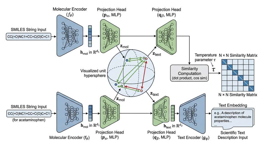
Alignment introduces projection heads \(p_\alpha: \mathbb{R}^{d_1} \to \mathbb{R}^{d}\) and \(q_\beta: \mathbb{R}^{d_2} \to \mathbb{R}^{d}\) that map both modalities into a shared \(d\)-dimensional space. After training, the projected embeddings \(\mathbf{z}^{(\text{mol})} = p_\alpha(f_\theta(x^{(\text{mol})}))\) and \(\mathbf{z}^{(\text{text})} = q_\beta(g_\phi(x^{(\text{text})}))\) satisfy a key property: if the molecule and text are semantically matched (the text describes the molecule), then \(\text{sim}(\mathbf{z}^{(\text{mol})}, \mathbf{z}^{(\text{text})})\) is high. If they are unmatched, the similarity is low. In short: alignment does not translate between modalities; it teaches two encoders to point in the same direction when they are talking about the same thing. Figure 28.1.1 illustrates the dual-encoder modality alignment architecture.

Contrastive Language-Image Pretraining (CLIP; Radford et al., 2021) introduced this paradigm by aligning images and text. The same architecture applies whenever paired cross-modal data exists: molecule-description pairs from PubChem, protein-function pairs from UniProt, image-caption pairs from scientific papers. The alignment objective is agnostic to the modalities; it requires only that paired examples be similar and unpaired examples be dissimilar.

Figure 28.1 illustrates the dual-encoder alignment architecture. Two pretrained encoders produce modality-specific embeddings, which projection heads then map into a shared vector space. The InfoNCE contrastive loss trains the projection heads (and optionally fine-tunes the encoders) so that matched pairs converge while unmatched pairs repel.

2. The InfoNCE Contrastive Loss

Without a principled training objective, projection heads learn arbitrary mappings that look aligned on training pairs but crumble on unseen molecules or descriptions. The loss function must do more than bring matched pairs closer; it must actively punish the model for confusing any molecule with any non-matching description in a large candidate pool, because real retrieval searches millions of candidates, not a handful.

The workhorse of modality alignment is the InfoNCE (Information Noise Contrastive Estimation) loss, introduced by van den Oord et al. (2018) and popularized by CLIP. Given a batch of \(N\) paired examples \(\{(x^{(\text{mol})}_i, x^{(\text{text})}_i)\}_{i=1}^{N}\), compute the projected embeddings \(\mathbf{z}^{(\text{mol})}_i\) and \(\mathbf{z}^{(\text{text})}_i\) for all \(i\). The loss treats the matching pair \((i, i)\) as the positive and all \(N-1\) non-matching pairs \((i, j)\) for \(j \neq i\) as negatives.

Define the similarity between the \(i\)-th molecule and the \(j\)-th text as:

where \(\tau > 0\) is a learnable temperature parameter. The molecule-to-text loss for sample \(i\) is a softmax cross-entropy over the similarity scores:

Symmetrically, the text-to-molecule loss treats row \(i\) of the transposed similarity matrix:

The total InfoNCE loss averages both directions:

Minimizing this loss forces the model to solve an \(N\)-way classification problem: given molecule \(i\), identify its matching text among \(N\) candidates (and vice versa). As \(N\) grows, the problem becomes harder and the representations must become more discriminative. This is why large batch sizes are typically important for contrastive learning; CLIP used batches of 32,768 pairs.

import torch
import torch.nn as nn
import torch.nn.functional as F


class InfoNCELoss(nn.Module):
    """
    Symmetric InfoNCE contrastive loss for cross-modal alignment.

    Given projected embeddings from two modalities, computes the
    bidirectional contrastive loss with learnable temperature.
    """

    def __init__(self, initial_temperature: float = 0.07):
        super().__init__()
        # Log-temperature is learnable; exp ensures tau > 0
        self.log_temperature = nn.Parameter(
            torch.log(torch.tensor(initial_temperature))
        )

    def forward(
        self,
        z_a: torch.Tensor,  # (batch, dim) from modality A
        z_b: torch.Tensor,  # (batch, dim) from modality B
    ) -> torch.Tensor:
        # L2-normalize embeddings to unit sphere
        z_a = F.normalize(z_a, dim=-1)
        z_b = F.normalize(z_b, dim=-1)

        # Cosine similarity matrix scaled by temperature
        temperature = self.log_temperature.exp()
        logits = z_a @ z_b.T / temperature  # (N, N)

        # Labels: diagonal entries are positive pairs
        labels = torch.arange(len(z_a), device=z_a.device)

        # Symmetric cross-entropy
        loss_a_to_b = F.cross_entropy(logits, labels)
        loss_b_to_a = F.cross_entropy(logits.T, labels)

        return (loss_a_to_b + loss_b_to_a) / 2

The InfoNCE loss defines what the model should optimize, but it says nothing about how embeddings from encoders with different architectures and dimensionalities arrive in a single shared space; that is the job of projection heads.

3. Projection Heads and Encoder Freezing

The projection heads \(p_\alpha\) and \(q_\beta\) are typically small multilayer perceptrons (MLPs) (two to three linear layers with ReLU or GELU activation, where GELU (Gaussian Error Linear Unit) is a smooth approximation of ReLU that weights inputs by their magnitude) that map encoder outputs to the shared space. Each encoder's forward pass produces a sequence of hidden states; the projection head takes a single pooled vector from that sequence (typically the CLS token, the first position's hidden state that transformer encoders learn to use as a whole-sequence summary) and maps it to the shared dimension. Their design involves several non-obvious choices.

Dimension of the shared space. CLIP uses \(d = 512\). Scientific multimodal models typically use \(d \in [256, 768]\). Larger \(d\) preserves more information but requires more data to fill the space usefully. Smaller \(d\) forces compression, which can improve generalization if the alignment signal is simple (e.g., matching a molecule to its name) but hurts if the relationship is nuanced (e.g., matching a molecule to a paragraph describing its mechanism of action).

Encoder freezing strategy. When the backbone encoders (\(f_\theta\) for molecules, \(g_\phi\) for text) are large pretrained models, you face a choice: freeze them and train only the projection heads, or fine-tune everything end-to-end. The tradeoffs parallel those in transfer learning (see Chapter 27). Freezing is computationally cheap and preserves the encoder's pretrained knowledge, but the projection heads alone may lack the capacity to bridge large representational gaps. End-to-end fine-tuning is more expressive but risks catastrophic forgetting, where the encoder loses its pretrained capabilities. A common compromise is staged training: freeze encoders for the first few epochs to warm up the projection heads, then unfreeze with a low learning rate.

import torch.nn as nn
from transformers import AutoModel, AutoTokenizer


class ProjectionHead(nn.Module):
    """
    Two-layer MLP projection head with layer normalization.

    Maps encoder hidden states to a shared embedding space
    for contrastive alignment.
    """

    def __init__(self, input_dim: int, projection_dim: int = 512):
        super().__init__()
        self.net = nn.Sequential(
            nn.Linear(input_dim, input_dim),
            nn.GELU(),
            nn.LayerNorm(input_dim),
            nn.Linear(input_dim, projection_dim),
        )

    def forward(self, x: torch.Tensor) -> torch.Tensor:
        return self.net(x)


class DualEncoderAligner(nn.Module):
    """
    Aligns two pretrained encoders via projection heads
    and InfoNCE contrastive loss.

    Parameters
    ----------
    encoder_a_name : str
        Hugging Face model name for modality A (e.g., molecular encoder).
    encoder_b_name : str
        Hugging Face model name for modality B (e.g., text encoder).
    projection_dim : int
        Dimension of the shared alignment space.
    freeze_encoders : bool
        If True, only projection heads are trained.
    """

    def __init__(
        self,
        encoder_a_name: str,
        encoder_b_name: str,
        projection_dim: int = 512,
        freeze_encoders: bool = True,
    ):
        super().__init__()
        self.encoder_a = AutoModel.from_pretrained(encoder_a_name)
        self.encoder_b = AutoModel.from_pretrained(encoder_b_name)

        dim_a = self.encoder_a.config.hidden_size
        dim_b = self.encoder_b.config.hidden_size

        self.proj_a = ProjectionHead(dim_a, projection_dim)
        self.proj_b = ProjectionHead(dim_b, projection_dim)
        self.loss_fn = InfoNCELoss()

        if freeze_encoders:
            for param in self.encoder_a.parameters():
                param.requires_grad = False
            for param in self.encoder_b.parameters():
                param.requires_grad = False

    def encode_a(self, **inputs) -> torch.Tensor:
        """Encode modality A inputs and project to shared space."""
        hidden = self.encoder_a(**inputs).last_hidden_state
        pooled = hidden[:, 0, :]  # CLS token pooling
        return self.proj_a(pooled)

    def encode_b(self, **inputs) -> torch.Tensor:
        """Encode modality B inputs and project to shared space."""
        hidden = self.encoder_b(**inputs).last_hidden_state
        pooled = hidden[:, 0, :]
        return self.proj_b(pooled)

    def forward(self, inputs_a: dict, inputs_b: dict) -> torch.Tensor:
        """Compute alignment loss for a batch of paired inputs."""
        z_a = self.encode_a(**inputs_a)
        z_b = self.encode_b(**inputs_b)
        return self.loss_fn(z_a, z_b)

4. Temperature Scaling and Its Effects

The temperature parameter \(\tau\) in the InfoNCE loss controls the sharpness of the softmax distribution over similarity scores. Its effect is both subtle and critical.

Low temperature (\(\tau \to 0\)) makes the softmax sharper: it assigns nearly all probability mass to the highest-similarity candidate. This forces the model to produce very distinct embeddings for non-matching pairs, which is good for retrieval precision but can lead to training instability (gradients become very large for hard negatives) and mode collapse, a degenerate state in which the model maps all inputs to the same region of the embedding space, erasing discriminative structure (the model pushes all negatives to exactly the same point).

High temperature (\(\tau \to \infty\)) makes the softmax uniform: every candidate gets similar probability regardless of actual similarity. This provides smooth gradients but weak learning signal; the model learns slowly and may converge to a suboptimal alignment.

CLIP initializes \(\tau = 0.07\) and learns it jointly with the model parameters. In practice, most scientific multimodal models follow this convention. The learned temperature typically converges to the range \([0.01, 0.1]\), depending on batch size and embedding dimension. A useful diagnostic: if \(\tau\) collapses to a very small value during training, the model is likely overfitting to easy negatives and needs harder ones.

Temperature controls how sharply the model discriminates among candidates, but discrimination is only as useful as the candidates themselves; if every negative in the batch is trivially different from the positive, even a well-tuned temperature cannot force the model to learn fine-grained distinctions.

5. Hard Negative Mining

Not all negative pairs are equally informative. A molecule for aspirin and a text describing a steel alloy are trivially distinguishable; the model learns nothing from pushing them apart. A molecule for aspirin and a text describing ibuprofen (another nonsteroidal anti-inflammatory drug, or NSAID, with similar properties) is a hard negative: the descriptions overlap significantly, and the model must learn subtle structural differences to distinguish them. Hard negatives drive the most learning.

In-batch negatives (the standard InfoNCE setup) provide some hard negatives by chance, but their difficulty depends on the batch composition. Several strategies increase the proportion of hard negatives:

• Pre-computed similarity mining. Before training, compute pairwise similarities across the dataset using the initial (pretrained) encoders. Construct batches where each positive pair is accompanied by its \(k\) nearest non-matching neighbors. This requires an offline index (Facebook AI Similarity Search (FAISS) or Scalable Nearest Neighbors (ScaNN); see Chapter 37) but dramatically improves alignment quality.
• Cross-batch memory banks. Maintain a queue of recent embeddings from previous batches. Each sample's negatives include not just the current batch but also the queue, effectively increasing the number of negatives without increasing batch size. Momentum Contrast (MoCo; He et al., 2020) popularized this approach.
• Curriculum-based hardness. Start training with easy negatives (random batches) and progressively increase hardness as the model improves. This avoids the instability that pure hard-negative mining can cause in early training.

import numpy as np
from dataclasses import dataclass


@dataclass
class HardNegativeBatchSampler:
    """
    Constructs batches with guaranteed hard negatives.

    For each anchor, includes its k nearest non-matching
    samples (by pre-computed embedding similarity) plus
    random negatives to fill the batch.

    Parameters
    ----------
    similarity_matrix : np.ndarray
        Pre-computed pairwise similarity, shape (N, N).
    k_hard : int
        Number of hard negatives per anchor.
    batch_size : int
        Total batch size (must be > k_hard + 1).
    """
    similarity_matrix: np.ndarray
    k_hard: int = 4
    batch_size: int = 32

    def __post_init__(self):
        n = len(self.similarity_matrix)
        # For each sample, rank others by similarity (descending)
        # Exclude self (diagonal)
        self.hard_negative_indices = np.zeros(
            (n, self.k_hard), dtype=np.int64
        )
        for i in range(n):
            sims = self.similarity_matrix[i].copy()
            sims[i] = -np.inf  # exclude self
            # Top-k most similar non-matching items
            top_k = np.argpartition(sims, -self.k_hard)[-self.k_hard:]
            self.hard_negative_indices[i] = top_k

    def sample_batch(self, anchor_idx: int) -> list[int]:
        """Build a batch around an anchor with hard negatives."""
        batch = {anchor_idx}
        # Add hard negatives
        for neg_idx in self.hard_negative_indices[anchor_idx]:
            batch.add(int(neg_idx))

        # Fill remaining slots with random samples
        n = len(self.similarity_matrix)
        while len(batch) < self.batch_size:
            rand_idx = np.random.randint(0, n)
            batch.add(rand_idx)

        return list(batch)[:self.batch_size]

# Using open_clip for contrastive alignment (15 lines vs 120)
import open_clip

model, preprocess_train, preprocess_val = open_clip.create_model_and_transforms(
    "ViT-B-32",  # or a custom architecture
    pretrained="laion2b_s34b_b79k",  # as of 2024, DataComp-trained checkpoints (e.g., "datacomp_xl_s13b_b90k") are preferred for new projects
)
tokenizer = open_clip.get_tokenizer("ViT-B-32")

# The library handles InfoNCE loss, temperature learning,
# gradient accumulation, and distributed training internally.
# Fine-tune on your domain pairs:
# open_clip.training.main(args)  # full training loop

6. Alignment Quality Metrics

Training a contrastive model is meaningless without measuring whether the alignment actually works. The standard metrics evaluate cross-modal retrieval: given a query in modality A, how well can you retrieve the correct match from modality B?

Recall@k measures the fraction of queries for which the correct match appears in the top \(k\) retrieved results:

where \(\text{rank}_i\) is the position of the true match for query \(i\) in the sorted list of candidates. Recall@1 is the most stringent (exact match at the top); Recall@10 is more lenient and commonly reported for scientific retrieval.

Mean Reciprocal Rank (MRR) gives credit to correct matches at any position, weighted by rank:

Alignment score (also called cross-modal cosine similarity) directly measures how close matched pairs are in the shared space. For a test set of \(M\) matched pairs:

A complementary metric is uniformity, which measures whether embeddings are spread evenly across the unit hypersphere (the surface of a sphere in \(d\)-dimensional space where every point has norm 1, which is where L2-normalized embeddings live) rather than collapsing to a small region. Good alignment requires both high alignment score (matched pairs are close) and high uniformity (unmatched pairs are spread out). Wang and Isola (2020) formalized this as the alignment-uniformity tradeoff.

import torch
import torch.nn.functional as F
from dataclasses import dataclass


@dataclass
class AlignmentMetrics:
    """
    Computes standard cross-modal alignment quality metrics.

    Parameters
    ----------
    z_a : torch.Tensor
        Projected embeddings from modality A, shape (N, d).
    z_b : torch.Tensor
        Projected embeddings from modality B, shape (N, d).
        Row i of z_b is the ground-truth match for row i of z_a.
    """
    z_a: torch.Tensor
    z_b: torch.Tensor

    def __post_init__(self):
        self.z_a = F.normalize(self.z_a, dim=-1)
        self.z_b = F.normalize(self.z_b, dim=-1)
        # Full similarity matrix: (N, N)
        self.sim_matrix = self.z_a @ self.z_b.T

    def recall_at_k(self, k: int = 10, direction: str = "a_to_b") -> float:
        """
        Fraction of queries where the true match is in the top-k.

        Parameters
        ----------
        k : int
            Number of top candidates to consider.
        direction : str
            "a_to_b" retrieves B given A; "b_to_a" retrieves A given B.
        """
        if direction == "a_to_b":
            sims = self.sim_matrix
        else:
            sims = self.sim_matrix.T

        n = sims.shape[0]
        # Get top-k indices for each query
        _, top_k_indices = sims.topk(k, dim=1)
        # True match for query i is index i
        targets = torch.arange(n, device=sims.device).unsqueeze(1)
        hits = (top_k_indices == targets).any(dim=1).float()
        return hits.mean().item()

    def mean_reciprocal_rank(self, direction: str = "a_to_b") -> float:
        """Average of 1/rank for the true match across all queries."""
        sims = self.sim_matrix if direction == "a_to_b" else self.sim_matrix.T
        n = sims.shape[0]
        # Rank of the true match (diagonal element)
        ranks = (sims >= sims.diag().unsqueeze(1)).sum(dim=1).float()
        return (1.0 / ranks).mean().item()

    def alignment_score(self) -> float:
        """Mean cosine similarity between matched pairs."""
        return self.sim_matrix.diag().mean().item()

    def uniformity(self, t: float = 2.0) -> float:
        """
        Uniformity loss (Wang & Isola, 2020).
        Lower is better (more uniform distribution on hypersphere).
        """
        sq_dists = torch.cdist(self.z_a, self.z_a, p=2).pow(2)
        return sq_dists.mul(-t).exp().mean().log().item()

    def report(self) -> dict:
        """Compute all standard metrics."""
        return {
            "recall@1_a2b": self.recall_at_k(1, "a_to_b"),
            "recall@5_a2b": self.recall_at_k(5, "a_to_b"),
            "recall@10_a2b": self.recall_at_k(10, "a_to_b"),
            "recall@1_b2a": self.recall_at_k(1, "b_to_a"),
            "recall@5_b2a": self.recall_at_k(5, "b_to_a"),
            "recall@10_b2a": self.recall_at_k(10, "b_to_a"),
            "mrr_a2b": self.mean_reciprocal_rank("a_to_b"),
            "mrr_b2a": self.mean_reciprocal_rank("b_to_a"),
            "alignment": self.alignment_score(),
            "uniformity": self.uniformity(),
        }

These metrics tell you how well alignment is working, but they also reveal when it is not; persistent low recall or collapsing uniformity are symptoms of specific, diagnosable failure modes.

When alignment succeeds. A well-aligned model shows three convergent signals during training: recall@10 climbs steadily across epochs (indicating that the correct match is consistently ranked near the top), alignment score increases without uniformity collapsing (indicating that matched pairs move closer without all embeddings collapsing to a single region), and the learned temperature \(\tau\) stabilizes rather than drifting toward zero or diverging. In downstream scientific applications, success means that free-text queries retrieve semantically correct molecules, proteins, or images from large candidate pools, enabling discovery workflows that would otherwise require hand-crafted domain-specific queries.

7. When Alignment Fails

Modality alignment is not guaranteed to work. Understanding the failure modes helps you diagnose and fix problems in practice.

Three Common Failure Modes

Modality gap. Even after alignment training, Liang et al. (2022) showed that CLIP-style models exhibit a persistent "modality gap": embeddings from different modalities occupy different regions of the shared space, separated by a constant offset. This gap means that cross-modal similarity scores are systematically lower than intra-modal scores, which can bias retrieval toward same-modality results if not accounted for.

Semantic granularity mismatch. A molecular structure encodes precise atomic connectivity, while a text description may operate at a coarse functional level ("anti-inflammatory agent"). Aligning these modalities at the wrong granularity leads to a space where similar descriptions map to dissimilar molecules. The solution is hierarchical alignment: separate losses for coarse-grained (drug class) and fine-grained (specific structure) matching.

Data quality. Contrastive alignment is only as good as the paired data. If the molecule-text pairs are noisy (the text describes the wrong molecule, or the description is too generic to be discriminative), the learned alignment will be noisy too. PubChem descriptions, the most commonly used source, vary enormously in specificity: some are detailed mechanistic descriptions, others are just "a chemical compound." Filtering for description quality before training is strongly recommended, because generic or incorrect descriptions introduce noise that the contrastive loss cannot distinguish from genuine semantic relationships.

8. Putting It Together: A Minimal Alignment Training Loop

The following example combines dual encoders, projection heads, InfoNCE loss, and alignment metrics in a complete training loop. It uses a toy dataset of molecule-text pairs but follows the same pattern that MoleculeSTM and similar production models use.

import torch
from torch.utils.data import DataLoader, Dataset
from typing import Iterator


class MoleculeTextDataset(Dataset):
    """
    Paired molecule SMILES and text descriptions.

    In production, load from PubChem or ChEBI.
    This example uses synthetic pairs for illustration.
    """

    def __init__(self, pairs: list[tuple[str, str]], tokenizer_a, tokenizer_b):
        self.pairs = pairs
        self.tok_a = tokenizer_a
        self.tok_b = tokenizer_b

    def __len__(self) -> int:
        return len(self.pairs)

    def __getitem__(self, idx: int) -> tuple[dict, dict]:
        smiles, text = self.pairs[idx]
        inputs_a = self.tok_a(
            smiles, return_tensors="pt", padding="max_length",
            max_length=128, truncation=True,
        )
        inputs_b = self.tok_b(
            text, return_tensors="pt", padding="max_length",
            max_length=256, truncation=True,
        )
        # Remove batch dim added by tokenizer
        return (
            {k: v.squeeze(0) for k, v in inputs_a.items()},
            {k: v.squeeze(0) for k, v in inputs_b.items()},
        )


def train_alignment(
    model: "DualEncoderAligner",
    train_loader: DataLoader,
    val_pairs: tuple[torch.Tensor, torch.Tensor],
    epochs: int = 20,
    lr: float = 1e-4,
) -> list[dict]:
    """
    Train a dual-encoder alignment model and track metrics.

    Parameters
    ----------
    model : DualEncoderAligner
        The alignment model with encoders and projection heads.
    train_loader : DataLoader
        Batches of paired (inputs_a, inputs_b) dictionaries.
    val_pairs : tuple
        Pre-computed (z_a_val, z_b_val) for validation metrics.
    epochs : int
        Number of training epochs.
    lr : float
        Learning rate for the optimizer.
    """
    optimizer = torch.optim.AdamW(
        [p for p in model.parameters() if p.requires_grad],
        lr=lr,
        weight_decay=0.01,
    )
    scheduler = torch.optim.lr_scheduler.CosineAnnealingLR(
        optimizer, T_max=epochs
    )

    history = []
    for epoch in range(epochs):
        model.train()
        total_loss = 0.0

        for inputs_a, inputs_b in train_loader:
            loss = model(inputs_a, inputs_b)
            optimizer.zero_grad()
            loss.backward()
            optimizer.step()
            total_loss += loss.item()

        scheduler.step()

        # Validation metrics
        model.eval()
        with torch.no_grad():
            metrics = AlignmentMetrics(*val_pairs).report()
            metrics["train_loss"] = total_loss / len(train_loader)
            metrics["epoch"] = epoch + 1
            metrics["temperature"] = model.loss_fn.log_temperature.exp().item()
            history.append(metrics)

        print(
            f"Epoch {epoch+1:3d} | "
            f"Loss: {metrics['train_loss']:.4f} | "
            f"R@10: {metrics['recall@10_a2b']:.3f} | "
            f"Align: {metrics['alignment']:.3f} | "
            f"tau: {metrics['temperature']:.4f}"
        )

    return history