37.1 RAG Architecture

"My context window is 200,000 tokens long, and I still cannot find my keys. Retrieval is about relevance, not capacity."

A Language Model With a Very Large, Very Disorganized Desk

1. The Three-Stage Pipeline

A researcher asks a language model which kinase inhibitors show synergy with immunotherapy in KRAS-mutant pancreatic cancer, and the model confidently names three compounds, complete with citation-shaped strings that lead nowhere, because every "fact" was fabricated from statistical patterns rather than retrieved from actual literature.

What. Retrieval Augmented Generation (RAG) is a design pattern that augments a language model's generation with evidence retrieved from an external knowledge base. Instead of relying on what the model memorized during pre-training, RAG fetches relevant documents at query time and includes them in the prompt.

Why. Language models trained on scientific literature have a knowledge cutoff date, cannot access proprietary corpora, and hallucinate with confidence. For scientific discovery, where correctness is non-negotiable and recency matters, retrieval provides a verifiable evidence trail that parametric memory cannot.

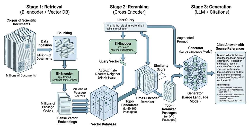
How. The pipeline processes a query through three stages, illustrated in Figure 37.1: (1) the retriever converts the query to a vector and finds candidate passages by similarity search, (2) the reranker scores each candidate with a more expensive cross-attention model and reorders them, and (3) the generator receives the top-ranked passages as context and produces a cited answer. Figure 37.1.1 illustrates the three-stage RAG pipeline architecture.

When. Use RAG when your corpus exceeds what fits in a single context window, when you need verifiable citations, when the corpus changes frequently, or when you must answer questions about proprietary documents the model has never seen.

The mathematical foundation is straightforward. Given a query \(q\) and a corpus of \(N\) passages \(\{p_1, p_2, \ldots, p_N\}\), the retriever computes a relevance score for each passage:

where \(\mathbf{e}_q\) and \(\mathbf{e}_{p_i}\) are dense vector embeddings and \(\text{sim}\) is typically cosine similarity (the dot product of two unit-length vectors, yielding a value between -1 and 1 that measures how closely the vectors point in the same direction) or inner product. The reranker then refines the top-\(k\) candidates with a cross-encoder score:

where \([q; p_i]\) denotes concatenation. The cross-encoder attends jointly to query and passage tokens, capturing fine-grained relevance that independent embeddings miss.

Mental Model

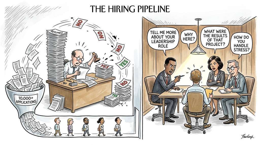
Think of the two stages like hiring at a large company. The bi-encoder is the resume screen: a recruiter reads each resume on its own and scores it against a job description, also read on its own. Because resumes and the job posting are evaluated independently, one recruiter can process thousands of applicants in a day. The cross-encoder is the panel interview: the candidate and the interviewers sit in the same room, and the conversation flows back and forth so that a follow-up question can probe exactly the claim on the resume that matters most. Interviews are far more accurate than resume screens, but you can only conduct a handful per day. No company interviews every applicant; instead it screens thousands down to a shortlist and interviews only those. RAG does the same: the bi-encoder screens millions of passages cheaply, and the cross-encoder "interviews" only the survivors.

2. Embedding Models for Scientific Text

The quality of a RAG system depends first on the quality of its embeddings. General-purpose embedding models (trained on web text, Wikipedia, and Stack Overflow) capture broad semantic similarity but often miss the nuances of scientific language. The phrase "inhibition of epidermal growth factor receptor (EGFR)" and "EGFR antagonism" are semantically identical to a domain expert but may land in distant regions of a general embedding space.

Several embedding models are well-suited to scientific retrieval. SPECTER2 (from the Allen Institute for AI) is trained on scientific paper abstracts and citation links. SciBERT provides domain-adapted embeddings for biomedical and computer science text. For general scientific use, modern models like E5-large-v2 and GTE-large offer strong performance across domains thanks to large-scale contrastive training (a learning paradigm that teaches the model to place semantically similar texts close together in embedding space while pushing dissimilar texts apart). As of 2025, newer embedding families have largely superseded these earlier models on the MTEB benchmark (Massive Text Embedding Benchmark, a standardized suite of tasks for evaluating embedding model quality across retrieval, classification, and clustering): BGE-M3 supports multilingual and multi-granularity retrieval, while GTE-Qwen2 and Cohere Embed v3 push accuracy further. The architectural principles remain the same.

The sentence-transformers library wraps these models with a consistent API, making the embedding stage straightforward to build. In short: the quality ceiling of every RAG system is set at indexing time; no reranker or generator can rescue passages that were poorly embedded.

from sentence_transformers import SentenceTransformer
import numpy as np

# Load a strong general-purpose embedding model
# For scientific corpora, consider 'allenai/specter2' instead
model = SentenceTransformer("BAAI/bge-large-en-v1.5")

# Scientific passages to index
passages = [
    "EGFR mutations in non-small cell lung cancer confer sensitivity "
    "to tyrosine kinase inhibitors such as erlotinib and gefitinib.",
    "The tumor suppressor p53 regulates apoptosis through both "
    "transcription-dependent and transcription-independent mechanisms.",
    "CRISPR-Cas9 enables precise genome editing by creating "
    "double-strand breaks at guide RNA-specified genomic loci.",
    "Transformer architectures process sequences through self-attention, "
    "computing pairwise interactions between all input tokens.",
    "Phase separation of intrinsically disordered proteins drives "
    "the formation of membraneless organelles in eukaryotic cells.",
]

# Compute embeddings (1024-dimensional vectors)
passage_embeddings = model.encode(
    passages,
    normalize_embeddings=True,  # Unit vectors for cosine similarity
    show_progress_bar=False,
    batch_size=32,
)

print(f"Embedding shape: {passage_embeddings.shape}")
print(f"Norm of first embedding: {np.linalg.norm(passage_embeddings[0]):.4f}")

# Query embedding
query = "What drugs target EGFR in lung cancer?"
query_embedding = model.encode(
    [query], normalize_embeddings=True
)

# Cosine similarity (dot product of unit vectors)
similarities = query_embedding @ passage_embeddings.T
ranked_indices = np.argsort(-similarities[0])

print(f"\nQuery: {query}")
for rank, idx in enumerate(ranked_indices[:3]):
    print(f"  Rank {rank+1} (sim={similarities[0][idx]:.4f}): "
          f"{passages[idx][:80]}...")

3. Vector Databases: Qdrant and pgvector

NumPy dot products work for a few thousand passages, but scientific corpora contain millions of papers with tens of millions of chunks. At that scale, you need a vector database that supports approximate nearest neighbor (ANN) search, metadata filtering, and persistent storage.

Approximate nearest neighbor (ANN) search finds vectors close to a query vector without comparing against every vector in the database. Exact nearest neighbor search scales linearly with the number of vectors. For corpora with tens of millions of chunks, each query would require billions of floating-point operations. ANN algorithms such as HNSW (Hierarchical Navigable Small World, a graph-based index structure that connects vectors to their approximate neighbors at multiple hierarchy levels for fast traversal) build a graph structure over the vectors during indexing. At query time, the search traverses only a small fraction of the graph, locating near-optimal neighbors in logarithmic time rather than linear time. Use ANN (via a vector database) whenever your corpus exceeds roughly 100,000 passages; below that threshold, exact brute-force search with NumPy or FAISS flat indices is simpler, fast enough, and guarantees perfect recall.

Two options cover most use cases. Qdrant is a purpose-built vector search engine with rich filtering, payload indexing, and both in-memory and on-disk storage modes. pgvector extends PostgreSQL with vector similarity search, ideal when your team already relies on PostgreSQL and wants to avoid a separate infrastructure dependency.

3.1 Indexing with Qdrant

from qdrant_client import QdrantClient
from qdrant_client.models import (
    Distance, VectorParams, PointStruct, Filter,
    FieldCondition, MatchValue
)

# In-memory client for development; use url="http://..." for production
client = QdrantClient(":memory:")

# Create a collection with cosine similarity
client.create_collection(
    collection_name="papers",
    vectors_config=VectorParams(
        size=1024,        # Embedding dimension
        distance=Distance.COSINE,
    ),
)

# Index passages with metadata
points = [
    PointStruct(
        id=i,
        vector=embedding.tolist(),
        payload={
            "text": passage,
            "source": f"paper_{i}.pdf",
            "year": 2023,
            "domain": domain,
        },
    )
    for i, (passage, embedding, domain) in enumerate(zip(
        passages, passage_embeddings,
        ["oncology", "oncology", "genomics", "ml", "cell_bio"]
    ))
]
client.upsert(collection_name="papers", points=points)

# Search with metadata filter: only oncology papers
results = client.query_points(
    collection_name="papers",
    query=query_embedding[0].tolist(),
    query_filter=Filter(
        must=[FieldCondition(key="domain", match=MatchValue(value="oncology"))]
    ),
    limit=3,
)

for result in results.points:
    print(f"Score: {result.score:.4f} | {result.payload['text'][:60]}...")

3.2 pgvector for PostgreSQL Teams

If your infrastructure already includes PostgreSQL, pgvector avoids the operational overhead of a separate vector database. It adds a vector column type and supports exact and approximate (IVFFlat, HNSW) nearest-neighbor search.

import psycopg2

# Connect to a PostgreSQL database with pgvector extension
conn = psycopg2.connect("postgresql://user:pass@localhost/papers_db")
cur = conn.cursor()

# Enable pgvector and create table
cur.execute("CREATE EXTENSION IF NOT EXISTS vector")
cur.execute("""
    CREATE TABLE IF NOT EXISTS paper_chunks (
        id SERIAL PRIMARY KEY,
        text TEXT NOT NULL,
        source TEXT,
        year INTEGER,
        domain TEXT,
        embedding vector(1024)
    )
""")

# Create HNSW index for fast approximate search
cur.execute("""
    CREATE INDEX IF NOT EXISTS paper_chunks_embedding_idx
    ON paper_chunks
    USING hnsw (embedding vector_cosine_ops)
    WITH (m = 16, ef_construction = 200)
""")

# Insert a passage
cur.execute(
    "INSERT INTO paper_chunks (text, source, year, domain, embedding) "
    "VALUES (%s, %s, %s, %s, %s)",
    (passages[0], "paper_0.pdf", 2023, "oncology",
     passage_embeddings[0].tolist())
)

# Query with cosine similarity, filtered by domain
cur.execute("""
    SELECT text, 1 - (embedding <=> %s::vector) AS similarity
    FROM paper_chunks
    WHERE domain = 'oncology'
    ORDER BY embedding <=> %s::vector
    LIMIT 5
""", (query_embedding[0].tolist(), query_embedding[0].tolist()))

for row in cur.fetchall():
    print(f"Similarity: {row[1]:.4f} | {row[0][:60]}...")

conn.commit()
conn.close()

4. Cross-Encoder Reranking

With passages indexed and searchable at scale, the remaining bottleneck is not finding candidates but separating the genuinely relevant results from the merely similar ones.

Bi-encoder retrieval is fast but imprecise. Because the query and passage are encoded independently, the model cannot capture fine-grained interactions between them. A passage might score highly because it shares vocabulary with the query but actually discusses a different aspect of the topic.

Cross-encoder rerankers solve this by processing the query and each candidate passage together through a transformer that attends to both simultaneously. The cross-attention layers (layers where each token in the query can attend to every token in the passage, and vice versa) can detect subtle relevance signals: negation ("does not inhibit EGFR"), specificity ("in non-small cell lung cancer, not small cell"), and argumentative structure ("contrary to previous findings...").

from sentence_transformers import CrossEncoder

# Load a cross-encoder reranker
reranker = CrossEncoder("cross-encoder/ms-marco-MiniLM-L-12-v2")

# Candidate passages from the retriever (top-k bi-encoder results)
query = "What is the role of p53 in cancer cell death?"
candidates = [
    "The tumor suppressor p53 regulates apoptosis through both "
    "transcription-dependent and transcription-independent mechanisms.",
    "EGFR mutations in non-small cell lung cancer confer sensitivity "
    "to tyrosine kinase inhibitors such as erlotinib and gefitinib.",
    "p53 activates the intrinsic apoptotic pathway by upregulating "
    "pro-apoptotic BCL-2 family members BAX and PUMA.",
    "TP53 is the most frequently mutated gene in human cancers, "
    "with loss-of-function mutations found in over 50% of tumors.",
    "Caffeine inhibits ATR kinase activity, abrogating the G2/M "
    "checkpoint and sensitizing p53-deficient cells to DNA damage.",
]

# Score each (query, passage) pair
pairs = [(query, candidate) for candidate in candidates]
scores = reranker.predict(pairs)

# Rerank by cross-encoder score
ranked = sorted(zip(scores, candidates), reverse=True)
for rank, (score, text) in enumerate(ranked):
    print(f"  Rank {rank+1} (score={score:.4f}): {text[:70]}...")

# Cohere reranking in 4 lines (vs. ~15 for self-hosted)
import cohere
co = cohere.ClientV2("your-api-key")
response = co.rerank(
    model="rerank-v3.5",
    query=query,
    documents=candidates,
    top_n=3,
)
for result in response.results:
    print(f"  Rank {result.index}: score={result.relevance_score:.4f}")

5. Retrieval Metrics: Recall@k, MRR, and NDCG

You cannot improve what you do not measure. Retrieval quality is evaluated with three complementary metrics, each capturing a different aspect of system performance.

Recall@k measures the fraction of relevant documents that appear in the top-\(k\) results. For a query with \(R\) relevant documents in the corpus:

Recall@k answers: "Did we find everything?" A Recall@10 of 0.8 means 80% of relevant documents appear in the top 10 results. For RAG, high recall is critical because the generator can only cite what the retriever surfaces.

Mean Reciprocal Rank (MRR) measures how early the first relevant document appears:

where \(\text{rank}_i\) is the position of the first relevant document for query \(i\). MRR answers: "How quickly did we find something useful?" An MRR of 0.5 means the first relevant document appears at rank 2 on average.

Normalized Discounted Cumulative Gain (NDCG) measures the quality of the entire ranking, giving more credit to relevant documents that appear earlier:

where \(\text{rel}_i\) is the relevance grade of the document at rank \(i\) and \(\text{IDCG@}k\) is the Discounted Cumulative Gain (DCG) of the ideal ranking. NDCG supports graded relevance (highly relevant, somewhat relevant, not relevant), making it the most informative single metric for retrieval quality.

import numpy as np

def recall_at_k(retrieved_ids: list, relevant_ids: set, k: int) -> float:
    """Fraction of relevant documents found in top-k results."""
    found = len(set(retrieved_ids[:k]) & relevant_ids)
    return found / len(relevant_ids) if relevant_ids else 0.0

def mrr(retrieved_ids: list, relevant_ids: set) -> float:
    """Reciprocal rank of the first relevant document."""
    for rank, doc_id in enumerate(retrieved_ids, start=1):
        if doc_id in relevant_ids:
            return 1.0 / rank
    return 0.0

def ndcg_at_k(retrieved_ids: list, relevance_grades: dict, k: int) -> float:
    """Normalized Discounted Cumulative Gain at position k."""
    dcg = sum(
        relevance_grades.get(doc_id, 0) / np.log2(rank + 2)
        for rank, doc_id in enumerate(retrieved_ids[:k])
    )
    # Ideal DCG: sort all grades descending
    ideal_grades = sorted(relevance_grades.values(), reverse=True)[:k]
    idcg = sum(
        grade / np.log2(rank + 2)
        for rank, grade in enumerate(ideal_grades)
    )
    return dcg / idcg if idcg > 0 else 0.0

# Example: evaluate a retrieval result
retrieved = ["doc_3", "doc_1", "doc_7", "doc_2", "doc_5"]
relevant = {"doc_1", "doc_2", "doc_5"}
grades = {"doc_1": 3, "doc_2": 2, "doc_5": 1}  # Graded relevance

print(f"Recall@3: {recall_at_k(retrieved, relevant, 3):.3f}")   # 1/3
print(f"Recall@5: {recall_at_k(retrieved, relevant, 5):.3f}")   # 3/3
print(f"MRR:      {mrr(retrieved, relevant):.3f}")               # 1/2
print(f"NDCG@5:   {ndcg_at_k(retrieved, grades, 5):.3f}")

6. Long-Context vs. Retrieval: The Tradeoff

Knowing how to measure retrieval quality raises a prior question: is retrieval even necessary when modern language models can ingest enormous prompts in a single pass?

Context windows now range from 100,000 to 1,000,000 tokens, making this question concrete rather than hypothetical. The answer depends on four factors.

Four Axes of the Tradeoff

Cost. Processing 200,000 tokens typically costs on the order of 100x more than processing 2,000 tokens of retrieved context, depending on the model and provider. For a research copilot handling thousands of queries per day, the cost difference is substantial. Retrieval lets you pay for relevance, not volume.

Accuracy. Long-context models suffer from the "lost in the middle" effect (Liu et al., 2024): they tend to attend more reliably to information at the beginning and end of the context than to information in the middle. A 100-paper context window may contain the answer on page 47, but the model may miss it. A retriever that surfaces the right paragraph puts it front and center.

Latency. Time-to-first-token scales with context length. A 200,000-token prompt takes seconds to process; a 2,000-token prompt with retrieved passages responds in under a second.

Freshness. Retrieval indices can be updated incrementally as new papers are published. Long-context approaches require re-assembling the entire context for each query, making it hard to keep current.

7. Query Planning for Multi-Hop Questions

Once you have decided that retrieval suits your corpus, the next challenge is that a single query often cannot capture the full scope of a complex research question.

Scientific questions are rarely simple. "What evidence supports the hypothesis that gut microbiome composition influences response to PD-1 checkpoint inhibitors in melanoma patients?" requires finding papers on gut microbiome composition, papers on PD-1 inhibitor response, and papers that connect the two in the context of melanoma. No single retrieval query will surface all the relevant evidence.

Query planning decomposes a complex question into simpler sub-queries, retrieves evidence for each, and combines the results. This is the multi-hop pattern (a retrieval strategy where answering one sub-question produces context needed to formulate the next sub-question, chaining retrieval steps together) that separates research copilots from basic question answering (QA) systems.

import anthropic

client = anthropic.Anthropic()

def decompose_query(complex_question: str) -> list[str]:
    """Decompose a complex scientific question into retrieval sub-queries."""
    response = client.messages.create(
        model="claude-sonnet-4-20250514",
        max_tokens=1024,
        messages=[{
            "role": "user",
            "content": f"""Decompose this scientific question into 2-4 simpler
sub-queries that can each be answered by searching a scientific paper database.
Each sub-query should target a specific aspect of the question.

Question: {complex_question}

Return ONLY a JSON array of sub-query strings, nothing else.
Example: ["sub-query 1", "sub-query 2", "sub-query 3"]"""
        }],
    )
    import json
    return json.loads(response.content[0].text)

# Example decomposition
question = (
    "What evidence supports the hypothesis that gut microbiome "
    "composition influences response to PD-1 checkpoint inhibitors "
    "in melanoma patients?"
)
sub_queries = decompose_query(question)
for i, sq in enumerate(sub_queries, 1):
    print(f"  Sub-query {i}: {sq}")

async def multi_hop_retrieve(
    question: str,
    retriever,  # Any retriever with a .search(query, k) method
    reranker,
    k_retrieve: int = 20,
    k_rerank: int = 5,
) -> dict:
    """Multi-hop retrieval: decompose, retrieve, rerank, deduplicate."""
    # Step 1: Decompose the question
    sub_queries = decompose_query(question)

    # Step 2: Retrieve candidates for each sub-query
    all_candidates = {}
    for sq in sub_queries:
        results = retriever.search(sq, k=k_retrieve)
        for doc_id, passage, score in results:
            if doc_id not in all_candidates:
                all_candidates[doc_id] = {
                    "passage": passage,
                    "retrieval_scores": {},
                }
            all_candidates[doc_id]["retrieval_scores"][sq] = score

    # Step 3: Rerank all unique candidates against the original question
    candidate_list = list(all_candidates.items())
    pairs = [(question, info["passage"]) for _, info in candidate_list]
    rerank_scores = reranker.predict(pairs)

    # Step 4: Combine and return top-k
    for (doc_id, info), score in zip(candidate_list, rerank_scores):
        info["rerank_score"] = float(score)

    ranked = sorted(
        candidate_list,
        key=lambda x: x[1]["rerank_score"],
        reverse=True,
    )[:k_rerank]

    return {
        "question": question,
        "sub_queries": sub_queries,
        "evidence": [
            {
                "doc_id": doc_id,
                "passage": info["passage"],
                "rerank_score": info["rerank_score"],
                "retrieval_scores": info["retrieval_scores"],
            }
            for doc_id, info in ranked
        ],
    }

8. The Generator: Producing Cited Answers

With retrieval and reranking supplying high-quality evidence, the remaining task is to synthesize that evidence into an answer the researcher can trust and trace back to its sources.

The generator is where evidence becomes answers. The prompt structure matters enormously for scientific RAG: the model must synthesize information from multiple passages, cite its sources, and refrain from adding information not present in the retrieved evidence.

def generate_cited_answer(
    question: str,
    evidence: list[dict],
    client: anthropic.Anthropic,
) -> str:
    """Generate a cited answer from retrieved evidence passages."""
    # Format evidence with source identifiers
    context_parts = []
    for i, ev in enumerate(evidence):
        context_parts.append(
            f"[Source {i+1}] (from {ev['doc_id']}, "
            f"relevance={ev['rerank_score']:.3f}):\n{ev['passage']}"
        )
    context = "\n\n".join(context_parts)

    response = client.messages.create(
        model="claude-sonnet-4-20250514",
        max_tokens=2048,
        system="""You are a scientific research assistant. Answer questions
based ONLY on the provided source passages. Follow these rules strictly:

1. Every factual claim must cite its source as [Source N].
2. If multiple sources support a claim, cite all of them.
3. If the sources do not contain enough information to answer
   the question fully, say so explicitly.
4. Do not add information from your training data. Only use
   what appears in the provided sources.
5. Distinguish between what the sources state directly and
   what you infer from combining multiple sources.""",
        messages=[{
            "role": "user",
            "content": f"""Based on the following source passages, answer
this research question:

Question: {question}

Sources:
{context}

Provide a detailed, cited answer."""
        }],
    )
    return response.content[0].text

This generator prompt is deliberately restrictive. In scientific contexts, an answer that cites a non-existent fact is worse than no answer at all. The instruction to "say so explicitly" when evidence is insufficient is critical: it converts the model's tendency to confabulate into an honest acknowledgment of gaps. We will formalize this as a measurable property (faithfulness) in Section 37.2.

Section Summary

The RAG pipeline transforms a language model from a closed-world system (limited to training data) into an open-world system that can answer questions about any corpus. The three stages (bi-encoder retrieval, cross-encoder reranking, constrained generation) each contribute a distinct capability: scale, precision, and synthesis. For scientific applications, the key architectural decisions are embedding model selection (domain-specific models typically outperform general ones), vector database choice (pgvector for existing PostgreSQL infrastructure, Qdrant for dedicated deployments), and the long-context versus retrieval tradeoff (retrieval wins for large, changing corpora; long context wins for deep analysis of small document sets). Query planning through decomposition enables multi-hop reasoning that single-query retrieval cannot achieve. The next section tackles the hardest remaining problem: ensuring that the generated answers are actually faithful to their sources.