Prerequisites
This section opens Part IV on knowledge-driven discovery. You should be comfortable with basic graph concepts (nodes, edges, adjacency matrices) from Chapter 3: Knowledge Representation and the search formalism from Chapter 1: Discovery as Search. Linear algebra basics (matrix multiplication, eigenvectors) from Appendix A will help with the PageRank derivation. Python proficiency with HTTP requests and JSON handling is assumed.
A citation is not just a reference; it is a vote of relevance, a trace of intellectual influence, and a link in the network of human knowledge. When we aggregate millions of these links into a graph, powerful patterns emerge: clusters of related work, bridging papers that connect disparate fields, and influential nodes that shaped entire research directions. This section teaches you to build and analyze citation networks at scale, using the same graph algorithms that power web search engines and social network analysis. By the end, you will be able to harvest metadata from open APIs, compute influence metrics, and automatically partition a research field into coherent topical communities. Figure 36.1 summarizes this end-to-end pipeline.
1. The Citation Network as a Directed Graph
In 2023, a computational biology lab spent four months pursuing a research direction they believed was novel, only to discover through automated citation analysis that a cluster of papers in a neighboring subfield had already solved the core problem. Without a structured way to map the literature, even careful researchers duplicate effort or miss critical connections. How did a single 1953 paper by Watson and Crick, just over one page long, end up shaping half a century of molecular biology while longer, more detailed contemporaries faded into obscurity? A citation network is a directed graph \(G = (V, E)\) where each node \(v \in V\) represents a paper and each directed edge \((u, v) \in E\) indicates that paper \(u\) cites paper \(v\). The direction encodes temporal information: the citing paper \(u\) was published after (or at least concurrently with) the cited paper \(v\). This makes citation networks approximately acyclic, though mutual citations between contemporaneous papers do create occasional cycles. Figure 36.1.1 illustrates citation network with PageRank influence propagation and Louvain community structure.
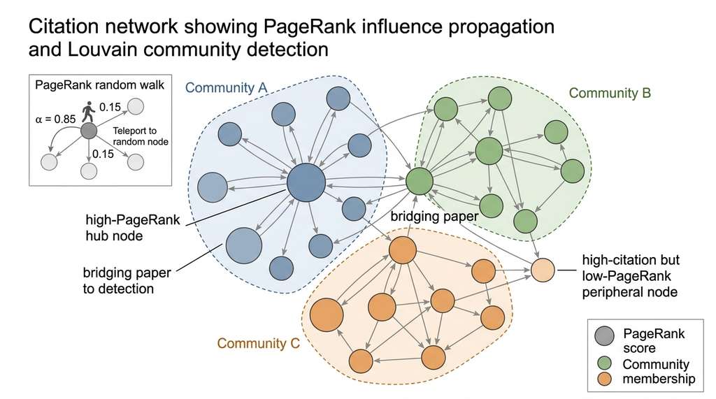
A citation network records which scholarly works acknowledge which predecessors, encoded as a graph that computational methods can operate on. It matters because no researcher can read an entire subfield's literature, often thousands of papers. The graph representation lets algorithms surface the most important works, detect topical clusters, and identify gaps in minutes rather than months. Each paper becomes a node. Each bibliographic reference becomes a directed edge from the citing paper to the cited one. Standard graph algorithms (shortest paths, centrality measures, community detection) then reveal structural patterns invisible to any individual reader. Use citation network analysis when you need a systematic, reproducible map of a research landscape; for targeted reading of a handful of known papers, a manual literature review remains sufficient.
The in-degree of a node (the number of papers that cite it) is the raw citation count, the simplest measure of a paper's impact. The out-degree (the number of references a paper makes) reflects the breadth of its literature review. Neither measure alone captures influence well. A paper cited 500 times by incremental follow-up studies is less influential than one cited 200 times across five different fields. To capture this distinction, we need network-aware metrics. In short: Count who cites you and you measure popularity; count who cites them and you begin to measure influence.
Common Misconception
A frequent mistake is equating a paper's citation count with its quality or importance. High citation counts can result from factors unrelated to scientific merit: a paper may be widely cited because it introduces a popular dataset, because it appears in a high-visibility venue, or because it contains an error that many subsequent papers need to address. Citation count measures attention, not correctness; to assess genuine influence, you need network-aware metrics like PageRank or betweenness centrality that account for who is doing the citing and how the paper connects different parts of the literature.
Citation networks exhibit strong preferential attachment (the tendency for highly cited papers to attract citations at a faster rate than less cited ones), clustering (papers in the same subfield cite each other densely), and aging effects (older papers accumulate citations over time but eventually stop being cited as the field moves on). These structural properties mean that naive statistical assumptions (uniform edge probability, independence of citations) produce misleading results. Every metric and algorithm in this section is designed to account for these real-world network properties.
2. Harvesting Scholarly Metadata at Scale
With the graph formalism in place, the next question is practical: where do the nodes and edges come from?
Building citation networks requires raw data. Three open APIs provide the raw material: OpenAlex (the successor to Microsoft Academic Graph, with 250+ million works (circa 2024)), Semantic Scholar (focused on computer science, biomedicine, and physics, with AI-generated features like too long; didn't read (TLDR) summaries and Scientific Paper Embeddings using Citation-informed TransformErs (SPECTER) embeddings), and Crossref (the Digital Object Identifier (DOI) registration agency, with 150+ million metadata records (circa 2024)). Each API has different strengths, rate limits, and data coverage.
OpenAlex serves as the primary data source here: it offers the broadest coverage, a generous free API, and rich citation metadata. The following client class handles pagination, rate limiting, and error recovery.
import time
import requests
from dataclasses import dataclass, field
from typing import Iterator


@dataclass
class Paper:
    """Minimal paper record from OpenAlex."""
    openalex_id: str
    doi: str | None
    title: str
    year: int | None
    cited_by_count: int
    abstract: str | None
    referenced_works: list[str] = field(default_factory=list)
    concepts: list[dict] = field(default_factory=list)


class OpenAlexClient:
    """Polite OpenAlex API client with pagination and rate limiting."""

    BASE_URL = "https://api.openalex.org"

    def __init__(self, email: str, per_page: int = 100):
        self.session = requests.Session()
        # OpenAlex asks for a contact email for the polite pool
        self.session.params = {"mailto": email, "per_page": per_page}
        self.per_page = per_page
        self._last_request_time = 0.0

    def _throttle(self):
        """Enforce at most 10 requests per second (polite pool)."""
        elapsed = time.time() - self._last_request_time
        if elapsed < 0.1:
            time.sleep(0.1 - elapsed)
        self._last_request_time = time.time()

    def search_works(
        self, query: str, filters: dict | None = None, max_results: int = 500
    ) -> Iterator[Paper]:
        """Search for works, yielding Paper objects with full pagination."""
        params = {"search": query}
        if filters:
            filter_str = ",".join(f"{k}:{v}" for k, v in filters.items())
            params["filter"] = filter_str

        cursor = "*"
        yielded = 0
        while cursor and yielded < max_results:
            self._throttle()
            params["cursor"] = cursor
            resp = self.session.get(f"{self.BASE_URL}/works", params=params)
            resp.raise_for_status()
            data = resp.json()

            for item in data.get("results", []):
                if yielded >= max_results:
                    break
                yield self._parse_work(item)
                yielded += 1

            cursor = data.get("meta", {}).get("next_cursor")

    def _parse_work(self, item: dict) -> Paper:
        """Convert an OpenAlex work record to our Paper dataclass."""
        # Extract abstract from inverted index if available
        abstract = None
        if inv_index := item.get("abstract_inverted_index"):
            abstract = self._reconstruct_abstract(inv_index)

        return Paper(
            openalex_id=item["id"],
            doi=item.get("doi"),
            title=item.get("title", ""),
            year=item.get("publication_year"),
            cited_by_count=item.get("cited_by_count", 0),
            abstract=abstract,
            referenced_works=item.get("referenced_works", []),
            concepts=[
                {"name": c["display_name"], "score": c["score"]}
                for c in item.get("concepts", [])
                if c.get("score", 0) > 0.3
            ],
        )

    @staticmethod
    def _reconstruct_abstract(inv_index: dict) -> str:
        """Reconstruct abstract text from OpenAlex inverted index format."""
        positions = []
        for word, indices in inv_index.items():
            for idx in indices:
                positions.append((idx, word))
        positions.sort()
        return " ".join(word for _, word in positions)


# Usage: harvest papers on a topic
client = OpenAlexClient(email="researcher@university.edu")
papers = list(client.search_works(
    query="large language models scientific discovery",
    filters={"publication_year": ">2020", "type": "article"},
    max_results=500,
))
print(f"Harvested {len(papers)} papers")
concepts field in favor of a richer topics taxonomy; production code should migrate to item.get("topics", []) and adjust the filtering key accordingly.A materials science team wanted to map the landscape of perovskite solar cell research. They compared three APIs: OpenAlex returned 12,400 papers with full citation links but sparse abstracts (about 60% coverage). Semantic Scholar returned 8,200 papers but included SPECTER embeddings and AI-generated TLDRs for each one. Crossref returned 15,000 DOI records but without citation links (only reference lists embedded in metadata). The team used OpenAlex for the citation network structure, Semantic Scholar for embeddings and semantic search, and Crossref for DOI validation and publisher metadata. This multi-source strategy, harvesting complementary data from each API, is the standard approach for production literature mining.
3. Bibliometric Indicators
Once the raw citation data is in hand, the natural next step is to measure what it tells us about individual papers and researchers.
Raw citation counts are a blunt instrument. A paper with 1,000 citations in a field where the median is 50 is far more exceptional than one with 1,000 citations where the median is 500. Bibliometrics, the quantitative study of scholarly publications and their citation patterns, provides a family of normalized, context-aware indicators that quantify impact more meaningfully.
3.1 The h-index
The h-index (Hirsch, 2005) is the largest integer \(h\) such that a researcher has at least \(h\) papers with at least \(h\) citations each. Formally, given a list of citation counts \(c_1 \geq c_2 \geq \cdots \geq c_n\) sorted in descending order:
$$h = \max\{i : c_i \geq i\}$$The h-index balances productivity and impact: a researcher with one paper cited 10,000 times (and nothing else) has \(h = 1\), while a researcher with 50 papers each cited 50 times has \(h = 50\). Its simplicity is both its strength and its weakness. The h-index cannot decrease over time, penalizes early-career researchers, and ignores the distribution shape beyond the threshold. Variants like the g-index (which gives more weight to highly cited papers) and the i10-index (count of papers with 10+ citations) address some of these limitations.
import numpy as np


def h_index(citation_counts: list[int]) -> int:
    """Compute the h-index from a list of citation counts."""
    sorted_counts = sorted(citation_counts, reverse=True)
    h = 0
    for i, count in enumerate(sorted_counts, start=1):
        if count >= i:
            h = i
        else:
            break
    return h


def g_index(citation_counts: list[int]) -> int:
    """Compute the g-index: largest g where top-g papers have >= g^2 total cites."""
    sorted_counts = sorted(citation_counts, reverse=True)
    cumsum = np.cumsum(sorted_counts)
    g = 0
    for i in range(1, len(sorted_counts) + 1):
        if cumsum[i - 1] >= i * i:
            g = i
        else:
            break
    return g


# Example: compute for a researcher's publication record
cites = [245, 112, 89, 67, 45, 32, 28, 15, 8, 3, 1, 0]
print(f"h-index: {h_index(cites)}")   # h = 7
print(f"g-index: {g_index(cites)}")   # g = 10 (top 10 sum to 644 >= 100)
3.2 Citation Half-Life and Aging
The citation half-life of a paper is the time at which it has received half of its total citations to date. Fields with short half-lives (computer science, around 5 years) evolve rapidly; fields with long half-lives (mathematics, around 15 years) build on older work more persistently. For a collection of papers, we compute the median citation age:
$$\tau_{1/2} = \text{median}\{t_{\text{now}} - t_{\text{cite}} : (u, v) \in E, v \in S\}$$where \(S\) is the set of papers whose half-life we are measuring and \(t_{\text{cite}}\) is the publication year of each citing paper \(u\). Citation half-life helps literature miners calibrate their time windows: in a fast-moving field, papers older than \(2\tau_{1/2}\) may no longer represent the state of the art.
Checkpoint
So far: raw citation count measures attention but not quality; the h-index balances productivity and impact, the g-index gives more credit to highly cited papers, and citation half-life captures how quickly a field's references age.
4. PageRank for Scientific Influence
Raw citation count treats every citation equally. But a citation from a Nature review paper carries more weight than one from an obscure workshop abstract. PageRank (Page et al., 1999), originally developed for web search, captures this recursive definition of importance: a paper is important if it is cited by other important papers.
Given a citation graph with adjacency matrix \(A\) (where \(A_{ij} = 1\) if paper \(i\) cites paper \(j\)), the PageRank vector \(\mathbf{r}\) satisfies:
$$\mathbf{r} = \alpha \, M^T \mathbf{r} + \frac{1-\alpha}{N} \mathbf{1}$$where \(M\) is the row-normalized adjacency matrix (\(M_{ij} = A_{ij} / \sum_k A_{ik}\)), \(\alpha\) is the damping factor (typically 0.85), \(N\) is the number of nodes, and \(\mathbf{1}\) is the all-ones vector. The damping factor models a "random researcher" who follows citation links with probability \(\alpha\) and jumps to a random paper with probability \(1 - \alpha\). The PageRank vector is the stationary distribution (the unique probability vector that remains unchanged after further transitions) of this random walk. In practice, the vector is computed via power iteration, a method that repeatedly multiplies an initial guess by the transition matrix until the values converge to a stable solution.
Mental Model
Think of PageRank like reputation in a professional recommendation network. Imagine you are hiring for a job and every candidate comes with letters of recommendation. A letter from a well-respected leader in the field carries far more weight than one from someone nobody has heard of. Now imagine that "well-respected" is itself defined by who recommended them, and so on, recursively. PageRank works the same way: each citation is a recommendation, and the weight of that recommendation depends on how many weighted recommendations the citing paper itself received. The damping factor (0.85) is like saying "85% of the time I trust the recommendation chain, and 15% of the time I just pick a random candidate to evaluate fresh," which prevents a single chain of mutual recommendations from inflating scores without bound.
The key difference between citation count and PageRank is recursion. A paper cited 50 times by other highly cited papers will have a higher PageRank than one cited 200 times by papers that nobody else cites. This matches scientific intuition: a foundational method paper that spawned an entire subfield (even if few people cite it directly anymore) retains high PageRank because its intellectual descendants are themselves highly cited. In practice, the top-10 papers by PageRank in a citation network typically include the genuine field-defining contributions.
import networkx as nx


def build_citation_graph(papers: list[Paper]) -> nx.DiGraph:
    """Build a NetworkX directed graph from harvested papers."""
    G = nx.DiGraph()

    # Index papers by OpenAlex ID for fast lookup
    paper_ids = {p.openalex_id for p in papers}

    for paper in papers:
        G.add_node(paper.openalex_id, title=paper.title,
                   year=paper.year, cited_by_count=paper.cited_by_count)
        for ref_id in paper.referenced_works:
            if ref_id in paper_ids:  # Only internal edges
                G.add_edge(paper.openalex_id, ref_id)

    return G


def rank_papers_by_influence(G: nx.DiGraph, top_k: int = 20) -> list[dict]:
    """Rank papers using PageRank and compare with raw citation count."""
    # Compute PageRank on the citation graph
    pagerank = nx.pagerank(G, alpha=0.85)

    # Build comparison table
    results = []
    for node, pr_score in sorted(pagerank.items(), key=lambda x: -x[1])[:top_k]:
        data = G.nodes[node]
        results.append({
            "id": node,
            "title": data.get("title", "")[:80],
            "year": data.get("year"),
            "citations": data.get("cited_by_count", 0),
            "pagerank": round(pr_score, 6),
            "pr_rank": None,   # filled below
            "cite_rank": None,
        })

    # Assign ranks
    pr_sorted = sorted(results, key=lambda x: -x["pagerank"])
    cite_sorted = sorted(results, key=lambda x: -x["citations"])
    for i, r in enumerate(pr_sorted):
        r["pr_rank"] = i + 1
    for i, r in enumerate(cite_sorted):
        r["cite_rank"] = i + 1

    return pr_sorted


# Build and analyze
G = build_citation_graph(papers)
print(f"Citation graph: {G.number_of_nodes()} papers, {G.number_of_edges()} citations")
top_papers = rank_papers_by_influence(G)
for p in top_papers[:5]:
    print(f"  PR#{p['pr_rank']} (Cite#{p['cite_rank']}): {p['title']}")
5. Community Detection with Louvain
A citation network of 500+ papers is too large to interpret by inspection. Automatic partitioning algorithms divide the graph into clusters of densely interconnected papers. In a citation network, these clusters correspond to topical communities: groups of papers that cite each other far more than they cite papers outside the group.
The Louvain algorithm (Blondel et al., 2008) optimizes a quantity called modularity, which measures the density of edges within communities relative to a random graph with the same degree sequence (the list of how many connections each node has). For an undirected graph with adjacency matrix \(A\), total edge weight \(m\), and community assignment \(c\), modularity is:
$$Q = \frac{1}{2m} \sum_{ij} \left[ A_{ij} - \frac{k_i k_j}{2m} \right] \delta(c_i, c_j)$$where \(k_i\) is the degree of node \(i\) and \(\delta(c_i, c_j) = 1\) if nodes \(i\) and \(j\) are in the same community. Values of \(Q\) above 0.3 generally indicate strong community structure. Louvain maximizes \(Q\) through a greedy, hierarchical process. First, each node starts as its own community. The algorithm then moves nodes to neighboring communities that yield the largest modularity gain. Finally, it collapses the resulting communities into super-nodes and repeats.
For citation networks, we convert the directed graph to undirected (treating a citation in either direction as a connection) because modularity is defined for undirected graphs and we care about topical relatedness, not citation direction.
from community import community_louvain  # python-louvain package
import collections


def detect_topic_communities(G: nx.DiGraph, resolution: float = 1.0) -> dict:
    """Detect topical communities in a citation network using Louvain.

    Returns a dict mapping community_id to list of paper IDs.
    """
    # Convert to undirected for community detection
    G_undirected = G.to_undirected()

    # Remove isolated nodes (no internal citations)
    isolates = list(nx.isolates(G_undirected))
    G_undirected.remove_nodes_from(isolates)

    # Run Louvain community detection
    partition = community_louvain.best_partition(
        G_undirected, resolution=resolution, random_state=42
    )

    # Group papers by community
    communities = collections.defaultdict(list)
    for node_id, comm_id in partition.items():
        communities[comm_id].append(node_id)

    # Compute modularity score
    Q = community_louvain.modularity(partition, G_undirected)
    print(f"Modularity Q = {Q:.3f} ({len(communities)} communities)")

    return dict(communities)


def label_communities(
    communities: dict, G: nx.DiGraph, papers_by_id: dict
) -> list[dict]:
    """Label each community by its most common concepts and top-cited paper."""
    community_info = []
    for comm_id, member_ids in sorted(communities.items(),
                                       key=lambda x: -len(x[1])):
        # Aggregate concepts across community members
        concept_counts = collections.Counter()
        top_paper = None
        top_cites = -1
        for pid in member_ids:
            paper = papers_by_id.get(pid)
            if paper:
                for c in paper.concepts:
                    concept_counts[c["name"]] += 1
                if paper.cited_by_count > top_cites:
                    top_cites = paper.cited_by_count
                    top_paper = paper

        community_info.append({
            "id": comm_id,
            "size": len(member_ids),
            "top_concepts": [c for c, _ in concept_counts.most_common(5)],
            "top_paper": top_paper.title if top_paper else "Unknown",
            "member_ids": member_ids,
        })

    return community_info


# Detect and label communities
communities = detect_topic_communities(G)
papers_by_id = {p.openalex_id: p for p in papers}
community_info = label_communities(communities, G, papers_by_id)
for c in community_info[:5]:
    print(f"Community {c['id']} ({c['size']} papers): {c['top_concepts'][:3]}")
leidenalg Python package provides a drop-in replacement via leidenalg.find_partition().A research group used the pipeline above to harvest 800 papers on "large language models for scientific discovery" from OpenAlex. Louvain community detection (at resolution 1.0) partitioned the citation graph into 12 communities with modularity \(Q = 0.42\), indicating strong topical structure. The five largest communities corresponded to: (1) LLMs for drug discovery and molecular generation (187 papers), (2) LLM-based code generation for scientific computing (134 papers), (3) retrieval-augmented generation (RAG) for literature synthesis (112 papers), (4) LLMs for materials property prediction (89 papers), and (5) autonomous research agents (67 papers). The smallest communities included niche applications in climate modeling and genomics. By examining the bridging papers (those with high betweenness centrality connecting two communities), the team identified a gap: very few papers connected the code generation community with the drug discovery community, suggesting an opportunity for tools that generate molecular simulation code.
6. Betweenness Centrality and Bridging Papers
While PageRank identifies the most influential papers within the network, betweenness centrality identifies papers that serve as bridges between different research communities. A paper with high betweenness centrality lies on many shortest paths between pairs of other papers, meaning it connects otherwise disconnected clusters. These bridging papers are often review articles, methods papers adopted across fields, or breakthrough results that opened new application domains.
For a node \(v\), betweenness centrality is:
$$C_B(v) = \sum_{s \neq v \neq t} \frac{\sigma_{st}(v)}{\sigma_{st}}$$where \(\sigma_{st}\) is the total number of shortest paths from \(s\) to \(t\), and \(\sigma_{st}(v)\) is the number of those paths that pass through \(v\).
def find_bridging_papers(G: nx.DiGraph, top_k: int = 10) -> list[dict]:
    """Find papers that bridge different research communities."""
    G_undirected = G.to_undirected()

    # Betweenness centrality (normalized)
    betweenness = nx.betweenness_centrality(G_undirected, normalized=True)

    bridges = []
    for node, bc_score in sorted(betweenness.items(), key=lambda x: -x[1])[:top_k]:
        data = G.nodes[node]
        bridges.append({
            "id": node,
            "title": data.get("title", ""),
            "year": data.get("year"),
            "betweenness": round(bc_score, 6),
            "degree": G_undirected.degree(node),
        })

    return bridges


bridges = find_bridging_papers(G)
print("Top bridging papers (connecting research communities):")
for b in bridges[:5]:
    print(f"  BC={b['betweenness']:.4f} deg={b['degree']}: {b['title'][:70]}")
Every graph metric in this section (PageRank, Louvain community detection, betweenness centrality)
is a single function call in NetworkX. The manual implementations above exist to explain the
algorithms; in production, you would use nx.pagerank(G) (1 line vs. 15 for power
iteration), community_louvain.best_partition(G) (1 line vs. the full modularity
optimization loop), and nx.betweenness_centrality(G) (1 line vs. the shortest-paths
enumeration). For graphs larger than 100,000 nodes, consider igraph or
graph-tool, which provide C-optimized implementations that can run 10 to 50 times faster
than NetworkX on large networks, depending on graph structure and algorithm.
7. Structural Holes and Research Gap Detection
The most actionable output of citation analysis is finding structural holes: places where two communities share related concepts yet rarely cite each other. These gaps represent research opportunities ripe for cross-pollination, where relevant groups have not yet discovered each other's work.
We quantify structural holes using the inter-community citation density. For two communities \(C_a\) and \(C_b\), the expected number of cross-citations under a random model is:
$$E[e_{ab}] = \frac{|C_a| \cdot |C_b|}{N^2} \cdot |E|$$where \(|E|\) is the total number of edges and \(N\) is the total number of nodes. The structural hole score is the ratio of observed to expected cross-citations:
$$\text{gap}(a, b) = 1 - \frac{e_{ab}^{\text{observed}}}{E[e_{ab}]}$$A gap score near 1 between two concept-sharing communities marks a strong candidate for interdisciplinary research.
A gap score close to 1 indicates that two communities cite each other far less than expected, suggesting an under-explored connection. We combine this with concept overlap (do the communities share any of the same OpenAlex concept tags?) to filter for gaps that are not just structural artifacts but represent genuinely related work that is not cross-citing.
import itertools


def find_structural_holes(
    G: nx.DiGraph,
    communities: dict,
    community_info: list[dict],
    min_shared_concepts: int = 2,
) -> list[dict]:
    """Find research gaps: community pairs with shared concepts but few citations."""
    total_edges = G.number_of_edges()
    total_nodes = G.number_of_nodes()

    gaps = []
    for info_a, info_b in itertools.combinations(community_info, 2):
        ids_a = set(info_a["member_ids"])
        ids_b = set(info_b["member_ids"])

        # Count cross-citations
        cross_cites = sum(
            1 for u, v in G.edges()
            if (u in ids_a and v in ids_b) or (u in ids_b and v in ids_a)
        )

        # Expected cross-citations under random model
        expected = (len(ids_a) * len(ids_b) / total_nodes**2) * total_edges
        if expected < 1:
            continue

        gap_score = 1 - min(cross_cites / expected, 1.0)

        # Concept overlap
        concepts_a = set(info_a["top_concepts"])
        concepts_b = set(info_b["top_concepts"])
        shared = concepts_a & concepts_b

        if len(shared) >= min_shared_concepts and gap_score > 0.5:
            gaps.append({
                "community_a": info_a["id"],
                "community_b": info_b["id"],
                "size_a": info_a["size"],
                "size_b": info_b["size"],
                "cross_citations": cross_cites,
                "expected_citations": round(expected, 1),
                "gap_score": round(gap_score, 3),
                "shared_concepts": list(shared),
            })

    return sorted(gaps, key=lambda x: -x["gap_score"])
8. Visualizing the Citation Landscape
Structural holes and community labels are powerful analytical outputs, but communicating them to collaborators requires something more immediate than a table of numbers.
A table of community labels and gap scores is useful for computation but hard for humans to interpret. Visualization transforms the abstract graph into an intuitive map. We use a force-directed layout (where nodes repel each other like charged particles while edges act as springs, settling into positions that reflect graph structure) that places densely connected papers close together and separates weakly connected communities, then color-code by community membership.
import matplotlib.pyplot as plt
import matplotlib.cm as cm


def plot_citation_landscape(
    G: nx.DiGraph, partition: dict, output_path: str = "citation_landscape.jpg"
):
    """Visualize the citation network colored by Louvain communities."""
    G_undirected = G.to_undirected()

    # Remove isolates for cleaner visualization
    isolates = list(nx.isolates(G_undirected))
    G_vis = G_undirected.copy()
    G_vis.remove_nodes_from(isolates)

    # Force-directed layout
    pos = nx.spring_layout(G_vis, k=0.3, iterations=50, seed=42)

    # Color by community
    communities_present = set(partition[n] for n in G_vis.nodes())
    cmap = cm.get_cmap("tab20", len(communities_present))  # see note below for matplotlib 3.7+
    node_colors = [cmap(partition[n]) for n in G_vis.nodes()]

    # Size by citation count (log-scaled)
    sizes = [
        max(20, min(300, 10 * np.log1p(G.nodes[n].get("cited_by_count", 0))))
        for n in G_vis.nodes()
    ]

    fig, ax = plt.subplots(1, 1, figsize=(14, 10))
    nx.draw_networkx_nodes(
        G_vis, pos, node_color=node_colors, node_size=sizes, alpha=0.7, ax=ax
    )
    nx.draw_networkx_edges(G_vis, pos, alpha=0.05, ax=ax)
    ax.set_title("Citation Landscape: Communities by Color, Size by Citations")
    ax.axis("off")
    fig.tight_layout()
    fig.savefig(output_path, dpi=150, bbox_inches="tight")
    plt.close(fig)
    print(f"Saved citation landscape to {output_path}")
cm.get_cmap() is deprecated; use matplotlib.colormaps["tab20"] or plt.get_cmap("tab20") instead.Research Frontier
Classical bibliometric indicators assume that all citations carry equal semantic weight (endorsement, methodology reuse, criticism, or perfunctory background mention are all counted the same). Starting in 2019, Nicholson et al. developed scite Smart Citations and the accompanying Citation Statement Classification system, which uses transformer models trained on full-text citation contexts to classify each citation as "supporting," "contrasting," or "mentioning" the cited claim. Building on this, the 2024 system CiteAssist (Zhang et al., EMNLP 2024) demonstrated that replacing raw citation counts with sentiment-weighted citation scores substantially changes paper rankings: papers that receive many "contrasting" citations (indicating contested claims) drop in influence, while papers with high "supporting" ratios rise. Integrating citation intent classification into the PageRank framework taught in this section is an active area of research, with early results showing that intent-weighted PageRank correlates more strongly with expert assessments of paper quality than either raw citation count or standard PageRank.
Try It: Map a Research Field in 30 Minutes
Pick a research topic you care about and build a complete citation landscape using only a laptop and standard Python libraries. Follow these steps:
Step 1. Install the required packages: pip install requests networkx python-louvain matplotlib numpy.
Step 2. Use the OpenAlexClient class from Listing 36.1 to harvest 200 to 500 papers
on your chosen topic. Use your own email address in the constructor for the polite API pool. Filter
by publication_year to keep the results recent (e.g., ">2019").
Step 3. Build the citation graph with build_citation_graph() from Listing 36.3,
then compute PageRank. Print the top 10 papers by PageRank alongside their raw citation counts. Note
which papers rank differently under the two metrics and investigate why.
Step 4. Run Louvain community detection from Listing 36.4 and label each community by its
top concepts. Verify that the communities correspond to recognizable subtopics in your field. Experiment
with the resolution parameter (which controls how fine-grained the communities are: higher values produce more, smaller communities) by trying 0.5, 1.0, and 2.0 to see how it changes the granularity
of the partition.
Step 5. Run the structural hole analysis from Listing 36.6 to find community pairs with high gap scores and shared concepts. For the top gap, read the titles of the five most cited papers in each community and write one sentence describing the potential interdisciplinary connection that the gap suggests. This sentence is the seed for a new research question.
Exercise 36.1.1
A researcher has published 12 papers with the following citation counts (sorted in descending order):
[310, 95, 72, 60, 45, 40, 38, 12, 7, 3, 1, 0].
Compute (a) the h-index, (b) the g-index, and (c) explain why these two values differ. Then consider:
if the researcher publishes one new paper that immediately receives 50 citations, does the h-index
change? Does the g-index change? Why or why not?
Hint
For the h-index, walk down the sorted list and find the largest position i where the citation count is at least i. For the g-index, compute the cumulative sum of the sorted counts and find the largest g where that cumulative sum is at least g2. Remember that g-index rewards a few very highly cited papers more than h-index does.
Step-Through: PageRank Power Iteration
Trace through PageRank on a tiny 4-paper citation graph with damping factor \(\alpha = 0.85\). Papers A, B, C, D have these citation edges: B cites A, C cites A, C cites B, D cites C.
Initialization: \(r_A = r_B = r_C = r_D = 0.25\)
Iteration 1: Paper A is cited by B (B's only reference) and C (C has 2 references). So A receives \(0.85 \times (0.25/1 + 0.25/2) + 0.15/4 = 0.85 \times 0.375 + 0.0375 = 0.356\). Paper B is cited only by C (1 of C's 2 references): \(0.85 \times (0.25/2) + 0.0375 = 0.144\). Paper C is cited only by D (D's only reference): \(0.85 \times (0.25/1) + 0.0375 = 0.250\). Paper D is cited by nobody: \(0.85 \times 0 + 0.0375 = 0.0375\). After normalization: \(r_A = 0.452, r_B = 0.183, r_C = 0.317, r_D = 0.048\).
Iteration 2: Repeating with updated scores, A climbs further (\(r_A \approx 0.48\)) because both of its citers (B and C) themselves have nontrivial PageRank. D remains lowest because no paper cites it. After convergence (typically 20 to 50 iterations), the ranking stabilizes at A > C > B > D, matching our intuition that A is the foundational paper.
Real-World Application: OpenAlex in Elsevier's SciVal Platform
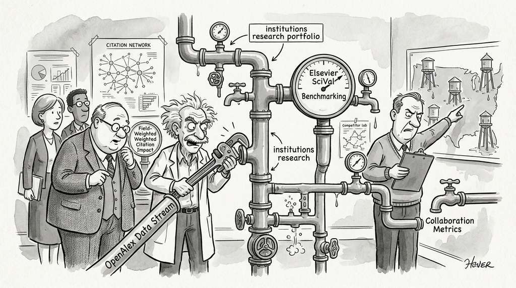
Elsevier's SciVal benchmarking platform uses citation network analysis (including field-weighted citation impact and collaboration metrics) to help universities evaluate their research portfolios against global peers. Institutions use these bibliometric dashboards to identify their strongest research clusters, track emerging fields, and allocate strategic funding. The underlying data pipeline harvests millions of citation links from Scopus and computes PageRank-family metrics at institutional scale, precisely the workflow this section teaches at the individual researcher level.
The Paper That Cites Itself 840 Times
In 2020, a team analyzing self-citation patterns discovered that a single paper in the biomedical literature contained over 840 citations to the first author's own prior work, inflating the author's h-index by an estimated 30 points. This extreme case led several funding agencies (including Italy's national research evaluation agency, ANVUR) to adopt "self-citation-adjusted" h-indices. The incident illustrates a broader lesson: any single-number metric will be gamed. Robust bibliometric analysis requires multiple complementary indicators (PageRank, betweenness centrality, community role) rather than reliance on any one score.
Lab: Build and Analyze a Real Citation Network
Goal: Harvest a citation network from OpenAlex, compute influence metrics, and detect topical communities for a research area of your choice.
Tools needed: Python 3.10+, requests, networkx,
python-louvain, matplotlib, numpy. No API key is required
(OpenAlex's polite pool only needs your email address).
Procedure (25 minutes): (1) Pick a focused topic (e.g., "graph neural networks
for drug discovery") and use the OpenAlexClient from Listing 36.1 to harvest 200 to
300 papers published after 2020. (2) Build the citation graph and compute both raw citation
rankings and PageRank. Record the top 10 papers under each metric. (3) Run Louvain community
detection at three resolution values (0.5, 1.0, 2.0) and note how the number and size of
communities change. (4) Run the structural hole analysis from Listing 36.6 and identify the
top-scoring gap.
What to vary: Try changing the harvest topic, the time window filter, and the Louvain resolution parameter. Compare your PageRank top-10 list against a Google Scholar search for the same topic.
What to observe: Do the PageRank and citation-count rankings agree on the top 5 papers, or do they diverge? At which resolution does Louvain produce communities that match recognizable subtopics in the field? Does the top structural hole correspond to a research gap you can articulate in one sentence?