Imagine handing a developer a 500,000-line codebase printed on paper, then covering all but 4% of the pages and asking them to fix a bug they cannot see. That is the situation every coding agent faces today. Modern large language models (LLMs) can process 128K to 1M tokens, yet production codebases routinely exceed 10 million tokens. Even if you could fit the entire repository into the context window, attention mechanisms degrade on long sequences, burying critical details in a sea of irrelevant code. The sections that follow quantify this mismatch, introduce the structural signals (file trees, import graphs, symbol tables) that help bridge the gap, and frame context selection as an optimization problem that the rest of this chapter solves.
1. The Scale Mismatch
A typical production codebase contains between 100,000 and 10,000,000 lines of code. At roughly 10 tokens per line of Python (accounting for indentation, operators, and identifiers), a 500,000-line repository consumes approximately 5,000,000 tokens. The largest commercially available context windows top out around 1,000,000 tokens (circa 2024, for models like Gemini 1.5 Pro). Most practical coding workflows use models with 128K to 200K token windows (as of 2025, Gemini 2.5 Pro and Claude 3.5 support windows of 1M and 200K tokens respectively, though the fundamental scale mismatch remains).
Context coverage measures the fraction of a codebase that fits into a single model prompt. This metric drives every design decision in this chapter. A coding agent can only reason about code it can see: if a critical dependency falls outside the coverage window, the agent will hallucinate interfaces, miss side effects, or produce patches that break at integration time. To compute coverage, divide the model's available token budget by the codebase's total token count; the result is the percentage of code visible in one interaction. When coverage exceeds 50%, pasting the file as a prompt suffices. When it drops below 10%, you need the retrieval and summarization pipeline described in the rest of this chapter. In short: the model can only reason about what it can see, and it can see at most a few percent of a real codebase.
Common Misconception
A frequent misconception is that a larger context window eliminates the need for context engineering. In practice, even a 1M-token window covers only 10-20% of a large codebase, and attention quality typically degrades before the window is full (as documented by Liu et al., 2024), so careful selection of which code to include remains essential regardless of window size.
The arithmetic is unforgiving. If your codebase is \(L\) lines and the model's context window is \(W\) tokens, the fraction of the codebase you can present in a single prompt is:
$$ \text{coverage} = \frac{W}{L \times \bar{t}} $$where \(\bar{t}\) is the average number of tokens per line. For a 500K-line codebase with \(\bar{t} = 10\) and \(W = 200{,}000\), coverage is \(200{,}000 / 5{,}000{,}000 = 4\%\). The agent sees at most 4% of the code in any single interaction. Choosing which 4% to show is the core challenge of context engineering.
import os
from pathlib import Path

def measure_codebase(root: str, extensions: set[str] = {".py"}) -> dict:
    """Count lines and estimate tokens for a codebase."""
    total_lines = 0
    total_files = 0
    tokens_per_line = 10  # empirical average for Python

    for path in Path(root).rglob("*"):
        if path.suffix in extensions and path.is_file():
            try:
                lines = path.read_text(encoding="utf-8").count("\n")
                total_lines += lines
                total_files += 1
            except (UnicodeDecodeError, PermissionError):
                continue

    estimated_tokens = total_lines * tokens_per_line
    return {
        "files": total_files,
        "lines": total_lines,
        "estimated_tokens": estimated_tokens,
    }

# Example: measure a real project
stats = measure_codebase("/path/to/your/project")
context_windows = [128_000, 200_000, 1_000_000]
for w in context_windows:
    coverage = w / max(stats["estimated_tokens"], 1)
    print(f"  {w:>10,} tokens -> {coverage:.1%} coverage")
The CPython repository (the reference Python implementation) contains roughly 640,000
lines of Python and C code. At 10 tokens per line, that is approximately 6.4 million
tokens. With a 200K token context window, a coding agent can see about 3.1% of
CPython in a single interaction. To fix a bug in the garbage collector, the agent
needs to select precisely the right 3.1%, which includes the GC implementation
(Modules/gcmodule.c), the object header definitions
(Include/object.h), relevant test files, and the issue description. Missing
any of these pieces leads to incorrect patches. Including the entire
Lib/ directory instead wastes 90% of the budget on unrelated standard library
modules.
2. Attention Decay and the Lost-in-the-Middle Problem
Even when the context window fits all the needed code, a subtler problem remains: attention quality degrades with sequence length. Liu et al. (2024) showed that language models attend most strongly to the beginning and end of the context, with sharp drops in the middle third. Concatenating files in arbitrary order wastes these high-attention positions on irrelevant content.
Mental Model
Think of the context window as a bookshelf where you are searching for a recipe. You naturally scan the first few books and the last few books on the shelf with care, but your eyes glaze over the ones in the middle. If someone shelves the cookbook you need dead center in a long row, you will likely miss it and grab something from the ends instead. The "lost in the middle" effect works the same way: the model's attention mechanism gives strong weight to tokens near the start and end of the sequence, while tokens in the interior receive diluted attention. Effective context engineering is therefore not just about choosing which books go on the shelf, but about placing the most important ones at the ends where they will actually be read.
The attention mechanism in a transformer computes, for each query token \(q\), a weighted sum over all key-value pairs. The weight assigned to position \(j\) by query at position \(i\) is:
$$ \alpha_{ij} = \frac{\exp(q_i \cdot k_j / \sqrt{d_k})}{\sum_{m=1}^{n} \exp(q_i \cdot k_m / \sqrt{d_k})} $$As sequence length \(n\) grows, the softmax denominator (the normalizing sum in the equation above, which ensures all attention weights add to 1) grows, and the attention weight on any individual position shrinks. Positional encodings (Rotary Position Embedding (RoPE), Attention with Linear Biases (ALiBi)) attempt to preserve locality, but empirically the U-shaped attention curve persists. The practical consequence: position within the context matters as much as presence in the context.
Checkpoint
So far: a coding agent can see only a small fraction of a real codebase (the scale mismatch), and even within that fraction, the model attends unevenly, favoring tokens near the start and end of the context over those in the middle (attention decay), so both what you include and where you place it determine the quality of the agent's reasoning.
Effective context engineering optimizes along three axes simultaneously: relevance (is this code related to the task?), position (is it placed where the model attends most strongly?), and density (does it carry maximum information per token?). Optimizing only relevance while ignoring position produces a context window where the most important code sits in the middle, precisely where the model attends least. Optimizing only density while ignoring relevance produces maximally compressed but irrelevant context. The context engineering pipeline we build in this chapter addresses all three dimensions.
Understanding where a model attends most strongly raises a natural follow-up question: what exactly is it attending to, and how much meaning does each token carry? The answer turns on the information density of code, which differs radically from natural language.
3. Information Density of Code Versus Prose
Code is not prose. A single line of code can carry the semantic weight of an entire
paragraph of natural language. The statement
scores = torch.einsum('bhid,bhjd->bhij', queries, keys) / math.sqrt(d_k)
encodes the scaled dot-product attention formula, references four tensors by name
(implying specific shapes), invokes Einstein summation notation, and normalizes by the
key dimension. Explaining this line in prose takes 50 or more words; the code itself
is 12 tokens. That roughly 4-to-1 compression ratio means every token of code wasted on irrelevant files costs about four times more information than wasting a token of prose.
This high information density has two consequences for context engineering. First,
removing even a single line can destroy comprehension: dropping an import statement
makes every reference to that module unresolvable. Second, summarizing code requires
understanding its semantics, not just its surface form. A naive text summarizer that
shortens "a function that sorts a list" to "a sorting function" loses nothing, but
shortening def topological_sort(graph: dict[str, set[str]]) -> list[str]
to "a sorting function" loses the critical fact that this is a topological sort on a
directed graph, not a comparison sort on a list.
def estimate_information_density(code: str, description: str) -> float:
    """Compare token counts between code and its natural-language description.

    A ratio > 1 means the code is more information-dense than prose.
    """
    # Rough tokenization: split on whitespace and punctuation
    import re
    tokenize = lambda text: re.findall(r'\w+|[^\w\s]', text)

    code_tokens = len(tokenize(code))
    desc_tokens = len(tokenize(description))

    return desc_tokens / max(code_tokens, 1)

# Example
code = "scores = torch.einsum('bhid,bhjd->bhij', q, k) / math.sqrt(d_k)"
description = (
    "Compute the scaled dot-product attention scores by taking the "
    "Einstein summation of the query tensor (batch, heads, seq_len, dim) "
    "with the key tensor, producing a (batch, heads, seq_i, seq_j) "
    "attention matrix, then dividing by the square root of the key dimension "
    "for numerical stability."
)
ratio = estimate_information_density(code, description)
print(f"Information density ratio: {ratio:.1f}x")
# Output: Information density ratio: 3.8xBecause each token of code carries so much semantic weight, selecting the right fragments is critical; but selection requires knowing where to look inside a large repository. Fortunately, every codebase ships with structural metadata that can guide that search.
4. Repository Structure as a Signal Source
Raw source code is not the only source of context. Every repository carries rich structural signals that a context engineering system can exploit. Three structures are particularly valuable: file trees, import graphs, and symbol tables.
4.1 File Trees
The directory hierarchy of a well-organized codebase encodes architectural intent.
Files in src/models/ likely contain model definitions; files in
tests/unit/ contain unit tests; files in src/api/routes/
contain HTTP endpoint handlers. A file tree summary, even without reading any file
contents, tells an agent where to look for specific functionality. This is the cheapest
signal to compute: a single os.walk call produces it.
from pathlib import Path

def build_file_tree(root: str, max_depth: int = 4,
                    skip: set[str] = {".git", "node_modules", "__pycache__", ".venv"}
                    ) -> str:
    """Build a compact file tree string for context injection."""
    lines = []
    root_path = Path(root)

    def walk(path: Path, depth: int, prefix: str = ""):
        if depth > max_depth:
            return
        entries = sorted(path.iterdir(), key=lambda p: (p.is_file(), p.name))
        dirs = [e for e in entries if e.is_dir() and e.name not in skip]
        files = [e for e in entries if e.is_file()]

        for d in dirs:
            lines.append(f"{prefix}{d.name}/")
            walk(d, depth + 1, prefix + "  ")
        for f in files:
            lines.append(f"{prefix}{f.name}")

    lines.append(f"{root_path.name}/")
    walk(root_path, 0, "  ")
    return "\n".join(lines)

# Typically costs 200-500 tokens for a medium project
tree = build_file_tree("/path/to/project")
print(tree)4.2 Import Graphs
Import statements form a directed graph where each node is a module and each edge
represents a dependency. This graph tells us which files are likely relevant together:
if the agent is editing src/pipeline.py, and that file imports from
src/transforms.py and src/validators.py, then those two files
are strong candidates for context inclusion. The import graph also reveals the most
connected modules (hubs), which are the files most likely to be relevant to any task.
import ast
from collections import defaultdict
from pathlib import Path

def build_import_graph(root: str) -> dict[str, set[str]]:
    """Extract the import dependency graph from a Python project."""
    graph = defaultdict(set)
    root_path = Path(root)

    for py_file in root_path.rglob("*.py"):
        module = str(py_file.relative_to(root_path)).replace("/", ".").replace("\\", ".")
        module = module.removesuffix(".py").removesuffix(".__init__")

        try:
            tree = ast.parse(py_file.read_text(encoding="utf-8"))
        except (SyntaxError, UnicodeDecodeError):
            continue

        for node in ast.walk(tree):
            if isinstance(node, ast.Import):
                for alias in node.names:
                    graph[module].add(alias.name)
            elif isinstance(node, ast.ImportFrom):
                if node.module and not node.module.startswith("."):
                    graph[module].add(node.module)
                elif node.module:  # relative import
                    # Resolve relative imports against the module path
                    parts = module.split(".")
                    level = node.level
                    if level <= len(parts):
                        base = ".".join(parts[:-level]) if level > 0 else module
                        resolved = f"{base}.{node.module}" if node.module else base
                        graph[module].add(resolved)

    return dict(graph)

# Find the most-imported modules (hubs)
graph = build_import_graph("/path/to/project")
import_counts = defaultdict(int)
for source, targets in graph.items():
    for target in targets:
        import_counts[target] += 1
hubs = sorted(import_counts.items(), key=lambda x: -x[1])[:10]
print("Top 10 most-imported modules:")
for module, count in hubs:
print(f" {module}: imported by {count} files")4.3 Symbol Tables
A symbol table maps every name (function, class, variable, constant) to its location
and type. This is the densest structural signal: knowing that validate_schema
is a function defined at line 142 of src/validators.py that accepts a
dict and returns a bool gives the agent enough information to
call the function correctly without reading its entire implementation. We build symbol
tables using tree-sitter, an incremental parsing library that produces concrete syntax trees for source code in dozens of languages, in Section 11.2, where they
serve double duty as both a retrieval index and a summarization input.
Recent systems go well beyond hand-crafted structural signals. RepoFusion (Shrivastava et al., 2023) trains a model to jointly attend to multiple retrieved code snippets, learning which combinations are most useful. CodePlan (Bairi et al., 2024) uses a repository-level dependency graph to plan multi-file edits, treating the entire repository as a structured planning problem. More recently, SWE-Search (Antoniades et al., 2024) frames repository-level code editing as a tree search problem with a value function learned from agent trajectories, achieving strong results on SWE-bench, a benchmark that evaluates coding agents on real GitHub issues from popular open-source projects, (circa 2024) by dynamically deciding which files to explore and which edits to attempt based on a Monte Carlo Tree Search (MCTS) strategy. The emerging pattern is treating the repository not as a bag of files but as a richly connected search space where structural signals guide exploration. We revisit graph-based representations in Chapter 38: Knowledge Graph Discovery.
5. The Context Budget as an Optimization Problem
When a coding agent selects the wrong 4% of a repository, the result is not a minor inconvenience; it is a patch that silently breaks production because the agent never saw the validation logic two directories away. Framing context selection as a formal optimization problem turns this guesswork into a principled, repeatable process.
With all three signal sources in hand (file contents, structural signals, and summarizations), we can frame context selection precisely. Given a task description \(q\), a set of candidate context items \(\mathcal{C} = \{c_1, c_2, \ldots, c_n\}\) (code chunks, file summaries, tree fragments), and a token budget \(B\), we want to select a subset \(S \subseteq \mathcal{C}\) that maximizes a relevance score while fitting within the budget:
$$ \max_{S \subseteq \mathcal{C}} \sum_{c \in S} \text{relevance}(c, q) \quad \text{subject to} \quad \sum_{c \in S} \text{tokens}(c) \leq B $$This is a variant of the 0-1 knapsack problem (a classic optimization problem in which you must choose which items to pack into a container of fixed capacity, maximizing total value without exceeding the weight limit). Each context item \(c_i\) has a "weight" (its token count) and a "value" (its relevance to the current task). The budget \(B\) is the knapsack capacity. When relevance scores are independent across items, a greedy algorithm that sorts by value-to-weight ratio and packs greedily achieves a \(\tfrac{1}{2}\)-approximation for the 0-1 knapsack. When items interact (e.g., including file A makes file B more valuable because A imports B), the objective becomes submodular (meaning each additional item's marginal value can only stay the same or decrease as the selected set grows); greedy maximization under a cardinality constraint then guarantees a \(1 - 1/e\) approximation (Nemhauser et al., 1978), and practical performance is typically much better. We implement this optimization in Section 11.3.
from dataclasses import dataclass

@dataclass
class ContextItem:
    """A candidate item for context inclusion."""
    id: str              # e.g., "src/models/transformer.py:TransformerBlock"
    content: str         # the actual code or summary text
    tokens: int          # token count
    relevance: float     # relevance score to the current query (0 to 1)

def greedy_knapsack(items: list[ContextItem], budget: int) -> list[ContextItem]:
    """Select context items using greedy value-density packing."""
    # Sort by relevance-per-token (value density), descending
    ranked = sorted(items, key=lambda c: c.relevance / max(c.tokens, 1), reverse=True)

    selected = []
    remaining_budget = budget
    for item in ranked:
        if item.tokens <= remaining_budget:
            selected.append(item)
            remaining_budget -= item.tokens

    return selected

# Example usage
items = [
    ContextItem("models/base.py:BaseModel", "class BaseModel: ...", 450, 0.92),
    ContextItem("utils/logging.py:setup", "def setup_logging(): ...", 120, 0.35),
    ContextItem("models/attention.py:MHA", "class MultiHeadAttention: ...", 380, 0.88),
    ContextItem("tests/test_model.py", "class TestBaseModel: ...", 600, 0.71),
    ContextItem("config.py:defaults", "DEFAULT_CONFIG = {...}", 200, 0.65),
]
selected = greedy_knapsack(items, budget=1000)
for item in selected:
print(f" [{item.tokens:>4} tok] {item.id} (relevance: {item.relevance:.2f})")You might expect that doubling the context window would double coding agent performance. Empirically, it does not. SWE-bench results (circa 2024) show diminishing returns beyond 32K tokens of well-selected context, because additional context dilutes attention on the critical files. A perfectly curated 32K context often outperforms a carelessly assembled 128K context. This is the paradox: the scarcer the budget, the more it forces careful selection, which turns out to be more important than raw capacity. Context engineering is the discipline of making scarcity productive.
6. A Taxonomy of Context Engineering Strategies
The rest of this chapter builds four complementary strategies that, together, form a complete context engineering pipeline. Figure 11.1 illustrates how these four stages connect: raw source files enter the chunker, chunks flow through the summarizer, queries hit the retriever, and the packer assembles the final context window. Each strategy addresses a different aspect of the bottleneck:
- Chunking (Section 11.2): Break source files into semantically meaningful units (functions, classes, blocks) that can be individually scored and selected. This converts the granularity problem (files are too big; lines are too small) into a tractable indexing problem.
- Summarization (Section 11.2): Compress code chunks into shorter representations (signatures, docstrings, natural-language summaries) that preserve enough information for relevance scoring while consuming fewer tokens.
- Retrieval (Section 11.3): Given a task description, rank all chunks and summaries by relevance using a combination of dense embeddings, sparse keyword matching, and structural signals.
- Packing (Section 11.3): Select the highest-ranked items that fit within the token budget, respecting dependencies (if you include a function, include its imports) and optimizing position (most relevant items at the beginning and end of the context).
These four strategies compose into a pipeline: raw code enters the chunker, chunks flow through the summarizer, queries hit the retriever, and the packer assembles the final context window. The repository intelligence layer of Section 11.4 implements this entire pipeline as a reusable service. Figure 11.1.1 illustrates Context coverage scale mismatch and knapsack packing pipeline.
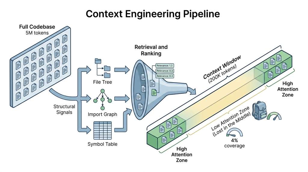
The open-source coding assistant Aider implements a "repository map" that builds a compact summary of the entire codebase using tree-sitter tags. In roughly 200 lines of Python, Aider extracts function and class definitions, computes a PageRank-style importance score (where PageRank is Google's algorithm for ranking nodes in a graph by the number and quality of links pointing to them) over the reference graph, and assembles a map that fits in 1,024 tokens. This single feature is credited by Aider's developers as a major contributor to its performance on SWE-bench. What takes us an entire chapter to build from first principles, Aider ships as a built-in feature. However, understanding the principles lets you customize the pipeline for domain-specific codebases (scientific code, embedded systems, polyglot repositories) where general-purpose tools fall short.
Try It: Measure and Visualize Your Own Context Budget
Pick any open-source Python project you have cloned locally and complete this five-step mini-project to internalize the scale mismatch firsthand.
- Run the
measure_codebasefunction from Listing 11.1 on the repository. Record the total file count, line count, and estimated token count. - Compute the coverage percentage for three context window sizes (128K, 200K, 1M tokens). Print the results as a small table.
- Use the
build_import_graphfunction from Listing 11.4 to extract the dependency graph. Identify the top five hub modules by in-degree (number of files that import them). - Using Python's
matplotlib, create a bar chart showing the top 10 hub modules and their import counts. Save it ascontext_hubs.png. - Estimate how many of those top-five hub files fit within a 32K-token budget by summing their line counts times 10 tokens per line. Write a one-paragraph reflection: does the budget leave room for the task-specific files an agent would also need?
Exercise 11.1.1
You are building a coding agent for a monorepo with 2,400 Python files totaling
360,000 lines. Your model offers a 200K token context window, and the system prompt
plus task description consume 8,000 tokens. The user asks the agent to refactor a
function in src/pipeline/transform.py, which imports from 12 other
internal modules (averaging 400 lines each). Calculate: (a) the effective token
budget available for code, (b) the total coverage percentage, and (c) whether the
12 imported modules alone fit within the budget. What does this tell you about the
necessity of summarization?
Hint
For (a), subtract the system prompt tokens from the window size. For (c), multiply 12 modules times 400 lines times 10 tokens per line and compare to your answer from (a). If the imports alone consume more than half the budget, the agent has little room left for the target file, tests, or structural signals.
Step-Through: Greedy Knapsack Context Packing
Trace through the greedy knapsack algorithm (Listing 11.5) with a budget of 700 tokens and these four candidate items:
- Item A: 300 tokens, relevance 0.90 (density = 0.90/300 = 0.0030)
- Item B: 150 tokens, relevance 0.60 (density = 0.60/150 = 0.0040)
- Item C: 400 tokens, relevance 0.85 (density = 0.85/400 = 0.00213)
- Item D: 200 tokens, relevance 0.70 (density = 0.70/200 = 0.0035)
Step 1: Sort by density (descending): B (0.0040), D (0.0035), A (0.0030), C (0.00213).
Step 2: Pack B. Budget remaining: 700 - 150 = 550. Total relevance: 0.60.
Step 3: Pack D. Budget remaining: 550 - 200 = 350. Total relevance: 1.30.
Step 4: Pack A. Budget remaining: 350 - 300 = 50. Total relevance: 2.20.
Step 5: Try C (400 tokens). Does not fit in 50 remaining. Skip.
Result: Selected {B, D, A} with total relevance 2.20 using 650 of 700 tokens.
Note that the greedy approach skipped Item C (the second most relevant by raw score)
because its information density was lowest.
Real-World Application: Sourcegraph Cody
Sourcegraph's AI coding assistant Cody uses a multi-signal context engine that combines the repository's code graph (symbols, references, call sites) with keyword search and embeddings to rank files before stuffing the prompt. In production deployments across enterprise codebases exceeding 10 million lines, Cody's context engine selects roughly 20 files per query, fitting them into a 32K token budget. This mirrors the knapsack framing from this section: the system scores each candidate file by relevance, weighs it by token cost, and packs greedily, confirming that careful selection at small budgets outperforms naive inclusion at large ones.
Lab: Mapping Your Own Context Budget
Goal: Empirically measure how context coverage varies across real
repositories and visualize where the token budget is spent.
Tools needed: Python 3.10+, tiktoken (for accurate GPT-style
token counting), matplotlib, and one or two cloned open-source repositories
(e.g., Flask at ~45K lines and CPython at ~640K lines).
Procedure (15-20 min):
- Install tiktoken:
pip install tiktoken. Use thecl100k_baseencoding to count tokens per file instead of the rough 10-tokens-per-line estimate (as of 2024, newer models such as GPT-4o use theo200k_baseencoding; choose the encoding that matches your target model). - For each repository, iterate over all
.pyfiles and record (file_path, line_count, token_count). Store the results in a list of tuples. - Sort files by token count descending. Plot a cumulative token curve (x = number of files included, y = cumulative tokens). Draw horizontal lines at 32K, 128K, and 200K to show how many files fit under each budget.
- What to vary: Try filtering to only the top-10 hub modules (by import in-degree from Listing 11.4) versus a random sample of 10 files. Compare cumulative token costs.
- What to observe: In most repositories, a small fraction of files (10-15%) accounts for over 50% of total tokens. Hub modules tend to be among the largest files, creating tension between their high relevance and their high token cost. This is exactly the trade-off the knapsack formulation captures.
Exercises
- (Conceptual) A repository has 1,200 Python files totaling 180,000 lines. Your model has a 128K token context window, and your system prompt and task description consume 4,000 tokens. Calculate the maximum coverage percentage. Then explain why even this coverage is an overestimate (hint: think about what else consumes tokens in a conversation).
-
(Coding) Run the
measure_codebasefunction from Listing 11.1 on a public repository of your choice (e.g., Flask, FastAPI, or scikit-learn). Build the import graph from Listing 11.4 and identify the top 5 hub modules. Explain why these modules would be strong default candidates for context inclusion. - (Analysis) The greedy knapsack in Listing 11.5 treats relevance scores as independent. Describe a scenario where including file A dramatically increases the value of including file B (i.e., relevance is submodular, not additive). How would you modify the greedy algorithm to account for this interaction?
What's Next
Context is the bottleneck, and structural signals can address it. In Section 11.2: Chunking and Summarization, we build the machinery that breaks source files into meaningful units and compresses them into context-efficient representations, using tree-sitter for parsing and both extractive and generative techniques for summarization.