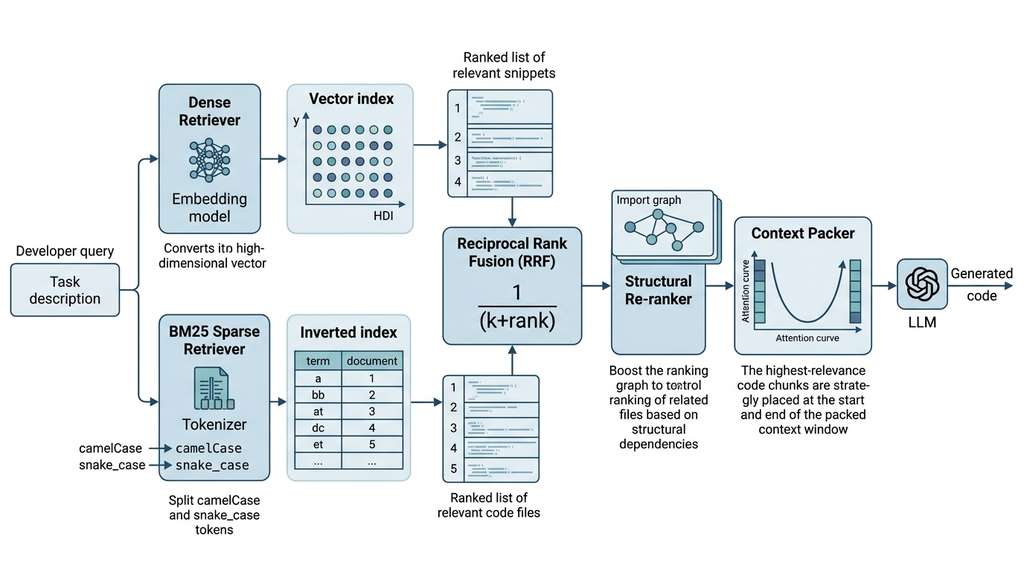
Section 11.2 produced a store of semantically chunked, summarized code units. This section builds the retrieval engine that, given a task description ("fix the pagination bug in the user list endpoint"), finds the chunks most likely to help. We combine three retrieval strategies: dense embedding search for semantic similarity, Best Matching 25 (BM25) for keyword matching, and structural re-ranking using import graphs. We then fuse results with Reciprocal Rank Fusion (RRF) and pack the winning chunks into the context window using the knapsack formulation from Section 11.1. The result is a retrieval-augmented code generation (RACG) pipeline that is the code-specific analog of the retrieval-augmented generation (RAG) systems covered in Chapter 37. Figure 11.3 illustrates how these stages connect into a single end-to-end pipeline.
1. Dense Retrieval with Code Embeddings
When a developer types "find the retry logic for API calls" and the system surfaces a function named _backoff_request from a file they have never opened, keyword matching cannot explain the result. Dense retrieval makes this leap by encoding both the query and every candidate chunk as vectors in a shared embedding space, then retrieving the \(k\) chunks whose vectors lie closest to the query vector. The quality of this approach depends entirely on the embedding model: it must map semantically similar code and natural-language descriptions to nearby points.
Dense retrieval converts natural-language queries and code fragments into fixed-length numerical vectors (embeddings), reducing semantic similarity to geometric proximity. A developer describes what they need in plain English ("find the retry logic for API calls") and retrieves relevant code even when no keywords overlap. An encoder neural network maps text to a point in high-dimensional space. A nearest-neighbor search then returns the \(k\) closest stored points. Use dense retrieval when queries describe intent or behavior. Switch to keyword-based methods (BM25, grep) when queries contain exact identifiers, error strings, or class names that must match literally.
Choosing an Encoder
Once you have committed to dense retrieval for an intent-based query, the critical engineering decision becomes which encoder to use, because the embedding model determines the geometry of that shared space.
General-purpose text embedding models (e.g., all-MiniLM-L6-v2) work
well on code because natural-language tokens in docstrings and variable names carry
semantic signal, but code-specialized models perform better. Models trained
on the CodeSearchNet benchmark (a dataset of six programming languages pairing functions with their docstrings, used to evaluate code search quality), such as microsoft/unixcoder-base and
Salesforce/codet5p-110m-embedding, learn to align code with its
natural-language description during pre-training (as of 2025, newer code embedding models such as Voyage AI's voyage-code-3 and OpenAI's text-embedding-3-large significantly outperform these earlier models on retrieval benchmarks, though the architectural principle of code-specialized pretraining remains the same). The cosine similarity between a
query "compute attention scores" and a function implementing scaled dot-product
attention should be high, even though the query and the code share few surface tokens.
The similarity between a query embedding \(\mathbf{q}\) and a chunk embedding \(\mathbf{c}\) is the cosine similarity:
$$ \text{sim}(\mathbf{q}, \mathbf{c}) = \frac{\mathbf{q} \cdot \mathbf{c}}{\|\mathbf{q}\| \cdot \|\mathbf{c}\|} $$For normalized embeddings (which most sentence-transformer models produce), this simplifies to the dot product \(\mathbf{q} \cdot \mathbf{c}\), making retrieval equivalent to a maximum inner product search (MIPS) problem (finding the stored vector whose dot product with the query vector is largest). In short: retrieval-augmented code generation turns "find the right file" from a human navigation problem into a geometry problem, where the best context is simply the nearest point.
import numpy as np
from sentence_transformers import SentenceTransformer

class DenseRetriever:
    """Embedding-based code retrieval using sentence-transformers."""

    def __init__(self, model_name: str = "all-MiniLM-L6-v2"):
        self.model = SentenceTransformer(model_name)
        self.chunks: list[dict] = []         # chunk metadata
        self.embeddings: np.ndarray | None = None  # (n_chunks, embed_dim)

    def index(self, chunks: list[dict]):
        """Embed and index a list of chunks.

        Each chunk dict must have 'id', 'content', and optionally
        'llm_summary' (preferred for embedding if available).
        """
        self.chunks = chunks

        # Prefer LLM summaries for embedding (better NL-to-NL matching)
        texts = []
        for c in chunks:
            if c.get("llm_summary"):
                texts.append(c["llm_summary"])
            elif c.get("signature"):
                texts.append(c["signature"])
            else:
                texts.append(c["content"][:2000])  # truncate long chunks

        self.embeddings = self.model.encode(
            texts, normalize_embeddings=True, show_progress_bar=True,
            batch_size=64,
        )

    def search(self, query: str, top_k: int = 20) -> list[tuple[dict, float]]:
        """Return top-k chunks ranked by cosine similarity to the query."""
        query_embedding = self.model.encode(
            [query], normalize_embeddings=True
        )[0]

        # Dot product = cosine similarity for normalized vectors
        scores = self.embeddings @ query_embedding
        top_indices = np.argsort(scores)[::-1][:top_k]

return [(self.chunks[i], float(scores[i])) for i in top_indices]Embedding the raw code of a 200-line class produces a single vector that averages over everything in the class. Embedding the LLM-generated summary of the same class produces a vector that captures its purpose, which is exactly what a natural-language query asks about. In retrieval benchmarks on CodeSearchNet (circa 2022), embedding summaries instead of raw code improves recall@10 by roughly 15 to 25 percent, regardless of the embedding model. This is why the summarization step in Section 11.2 is not merely a compression trick; it is a retrieval quality strategy.
2. Sparse Retrieval with BM25
Dense retrieval excels at semantic matching ("find functions related to authentication")
but struggles with exact identifier matching ("find all uses of
validate_jwt_token"). A query containing a specific function name, class
name, or error message needs lexical matching, not semantic similarity. This is where
BM25 shines.
BM25 is a probabilistic ranking function that extends term frequency-inverse document frequency (TF-IDF) with term frequency saturation (diminishing returns as a term repeats more often in a document) and document length normalization. For a query \(Q\) with terms \(q_1, \ldots, q_m\) and a document \(D\), the BM25 score is:
$$ \text{BM25}(D, Q) = \sum_{i=1}^{m} \text{IDF}(q_i) \cdot \frac{f(q_i, D) \cdot (k_1 + 1)}{f(q_i, D) + k_1 \cdot \left(1 - b + b \cdot \frac{|D|}{\text{avgdl}}\right)} $$where \(f(q_i, D)\) is the term frequency of \(q_i\) in \(D\), \(|D|\) is the document length, \(\text{avgdl}\) is the average document length across the corpus, \(k_1\) controls term frequency saturation (typically 1.2-2.0), and \(b\) controls length normalization (typically 0.75). The IDF (inverse document frequency) component is:
$$ \text{IDF}(q_i) = \ln\left(\frac{N - n(q_i) + 0.5}{n(q_i) + 0.5} + 1\right) $$where \(N\) is the total number of documents and \(n(q_i)\) is the number of documents containing term \(q_i\).
Checkpoint
So far: BM25 scores each chunk by how many query terms it contains, weighting rare terms (high IDF) more heavily while capping the benefit of repeated occurrences (saturation) and penalizing longer documents that match by sheer volume rather than focus.
from rank_bm25 import BM25Okapi
import re

class SparseRetriever:
    """BM25-based keyword retrieval for code chunks."""

    def __init__(self):
        self.chunks: list[dict] = []
        self.bm25: BM25Okapi | None = None

    @staticmethod
    def tokenize_code(text: str) -> list[str]:
        """Tokenize code for BM25: split on camelCase, snake_case, punctuation."""
        # Split camelCase: "validateJwtToken" -> ["validate", "Jwt", "Token"]
        text = re.sub(r'([a-z])([A-Z])', r'\1 \2', text)
        # Split on underscores and non-alphanumeric
        tokens = re.findall(r'[a-zA-Z]\w*', text.lower())
        return tokens

    def index(self, chunks: list[dict]):
        """Build the BM25 index from chunk contents."""
        self.chunks = chunks
        tokenized = [self.tokenize_code(c["content"]) for c in chunks]
        self.bm25 = BM25Okapi(tokenized)

    def search(self, query: str, top_k: int = 20) -> list[tuple[dict, float]]:
        """Return top-k chunks ranked by BM25 score."""
        query_tokens = self.tokenize_code(query)
        scores = self.bm25.get_scores(query_tokens)
        top_indices = np.argsort(scores)[::-1][:top_k]

        return [(self.chunks[i], float(scores[i])) for i in top_indices]
A developer reports a bug: "TypeError in UserSerializer.validate_email
when the input contains Unicode characters." This query contains a specific class
name, method name, and error type. BM25 immediately matches any chunk containing
UserSerializer and validate_email as tokens, scoring them
highly because these identifiers have high IDF (they appear in very few chunks).
A dense embedding model, by contrast, maps this query to the neighborhood of
"email validation" and "serialization," which is semantically correct but may rank
generic utility functions above the specific UserSerializer class. The
lesson: when the query contains specific identifiers, BM25 is the stronger signal.
When the query describes intent without naming specific code, embeddings win. Hybrid
search captures both.
3. Hybrid Search and Reciprocal Rank Fusion
When a coding agent retrieves context from the wrong combination of sources, the result is not merely suboptimal: the model generates code that confidently calls functions with incorrect signatures, references modules that do not exist in the repository, or misuses internal APIs whose contracts differ subtly from their public documentation. Getting retrieval fusion right is the difference between an agent that writes code against the real codebase and one that writes against a hallucinated approximation of it.
Neither dense nor sparse retrieval dominates in all cases. Hybrid search runs both retrievers in parallel and combines their rankings. The challenge is that dense scores (cosine similarity, range \([-1, 1]\)) and BM25 scores (unbounded positive reals) are not directly comparable. We need a rank-based fusion method that is agnostic to score scales. The five-stage flow in Figure 11.3 shows where RRF sits in this pipeline. Figure 11.3.1 illustrates Hybrid RACG pipeline with RRF fusion.
RRF (Cormack et al., 2009) is the standard solution. For each document \(d\), RRF computes a fused score based on the document's rank in each retriever's result list:
$$ \text{RRF}(d) = \sum_{r \in \mathcal{R}} \frac{1}{k + \text{rank}_r(d)} $$where \(\mathcal{R}\) is the set of retrievers, \(\text{rank}_r(d)\) is the rank of document \(d\) in retriever \(r\)'s results (1-indexed), and \(k\) is a constant (typically 60) that prevents the top-ranked result from dominating. If a document does not appear in a retriever's top-\(n\) results, its rank is set to \(n + 1\).
def reciprocal_rank_fusion(
    ranked_lists: list[list[tuple[dict, float]]],
    k: int = 60,
    top_n: int = 20,
) -> list[tuple[dict, float]]:
    """Fuse multiple ranked lists using Reciprocal Rank Fusion (RRF).

    Args:
        ranked_lists: list of ranked results from different retrievers,
                      each entry is (chunk_dict, score)
        k: RRF constant (default 60, per the original paper)
        top_n: number of results to return

    Returns:
        Fused ranking as (chunk_dict, rrf_score) pairs, descending.
    """
    rrf_scores: dict[str, float] = {}
    chunk_lookup: dict[str, dict] = {}

    for ranked_list in ranked_lists:
        for rank, (chunk, _score) in enumerate(ranked_list, start=1):
            chunk_id = chunk["id"]
            chunk_lookup[chunk_id] = chunk
            rrf_scores[chunk_id] = rrf_scores.get(chunk_id, 0.0) + 1.0 / (k + rank)

    # Sort by fused score, descending
    sorted_ids = sorted(rrf_scores.keys(), key=lambda cid: rrf_scores[cid], reverse=True)
    return [(chunk_lookup[cid], rrf_scores[cid]) for cid in sorted_ids[:top_n]]


class HybridRetriever:
    """Combines dense and sparse retrieval with RRF fusion."""

    def __init__(self, dense: DenseRetriever, sparse: SparseRetriever):
        self.dense = dense
        self.sparse = sparse

    def search(self, query: str, top_k: int = 20,
               dense_weight: int = 50, sparse_weight: int = 50) -> list[tuple[dict, float]]:
        """Hybrid search with configurable retriever candidate pool sizes."""
        dense_results = self.dense.search(query, top_k=dense_weight)
        sparse_results = self.sparse.search(query, top_k=sparse_weight)
return reciprocal_rank_fusion([dense_results, sparse_results], top_n=top_k)Mental Model
Think of reciprocal rank fusion as assembling a reading list from two librarians who each sort books by a different criterion: one by topic relevance, the other by how closely the title matches your exact words. You do not average their ratings (the scales are incompatible). Instead, you ask each librarian for a numbered ranking, then for every book you compute a score based solely on its position in each list. A book ranked 2nd by one librarian and 5th by the other earns \(1/(60+2) + 1/(60+5)\). The constant 60 acts like a "patience factor": it keeps a single first-place vote from drowning out consistent mid-rank appearances across both lists. The final reading list, sorted by combined position score, reflects agreement between the two ranking strategies without ever comparing their raw ratings.
4. Structural Re-ranking with Import Graphs
Hybrid search ranks chunks by textual relevance. But code has a structure that text does not: dependencies. If the agent is editing file A, and file A imports from file B, then chunks from file B are more likely to be relevant than chunks from an unrelated file C, even if C scores higher on textual similarity. (Structure beats semantics: a file one import edge away often outranks a file with a higher embedding score.) We exploit this by re-ranking results using the import graph from Section 11.1.
def structural_rerank(
    results: list[tuple[dict, float]],
    import_graph: dict[str, set[str]],
    focal_file: str | None = None,
    boost_factor: float = 1.5,
) -> list[tuple[dict, float]]:
    """Boost chunks from files that are structurally related to the focal file.

    A file is "structurally related" if it imports the focal file,
    is imported by the focal file, or shares an import with it.

    Args:
        results: ranked list from hybrid search
        import_graph: {module: {imported_modules}} from build_import_graph
        focal_file: the file being edited (if known)
        boost_factor: multiplicative boost for structurally related chunks

    Returns:
        Re-ranked results with structural boost applied.
    """
    if focal_file is None:
        return results

    # Normalize focal file to module path
    focal_module = focal_file.replace("/", ".").replace("\\", ".").removesuffix(".py")

    # Files imported by the focal file
    direct_imports = import_graph.get(focal_module, set())

    # Files that import the focal file (reverse edges)
    reverse_imports = {
        source for source, targets in import_graph.items()
        if focal_module in targets
    }

    # Co-imported files (share an import with focal file)
    co_imported = set()
    for source, targets in import_graph.items():
        if targets & direct_imports:  # shares at least one import
            co_imported.add(source)

    related = direct_imports | reverse_imports | co_imported

    # Apply boost
    boosted = []
    for chunk, score in results:
        chunk_module = (chunk["file_path"]
                        .replace("/", ".").replace("\\", ".")
                        .removesuffix(".py"))
        if chunk_module in related:
            boosted.append((chunk, score * boost_factor))
        else:
            boosted.append((chunk, score))

    boosted.sort(key=lambda x: x[1], reverse=True)
return boostedWith both textual relevance and structural proximity reflected in the scores, the pipeline's remaining challenge is fitting the winning chunks into a finite context window without exceeding the model's token budget.
5. Context Packing with Position Optimization
The final step takes the re-ranked chunks and packs them into the context window. Building on the greedy knapsack from Section 11.1, we add two refinements (both visible in Listing 11.18, which sorts candidates by relevance density, meaning the ratio of retrieval score to token cost, so that compact, high-value chunks are preferred). The first is dependency inclusion: if a chunk references a symbol defined in another chunk, include that chunk too. The second is position optimization: place the most relevant chunks at the beginning and end of the context, exploiting the U-shaped attention curve (the empirical finding that LLMs recall information placed at the start or end of the context window more reliably than information in the middle) from Liu et al., 2024.
from dataclasses import dataclass, field

@dataclass
class PackedContext:
    """The final assembled context window ready for LLM consumption."""
    items: list[dict] = field(default_factory=list)
    total_tokens: int = 0
    budget: int = 0

    def to_prompt(self) -> str:
        """Render the packed context as a prompt string."""
        sections = []
        for item in self.items:
            header = f"# {item['file_path']} :: {item['name']}"
            sections.append(f"{header}\n{item['content']}")
        return "\n\n".join(sections)


def pack_context(
    ranked_results: list[tuple[dict, float]],
    budget: int,
    chunk_store: "ChunkStore",
    include_parent_signatures: bool = True,
) -> PackedContext:
    """Pack ranked chunks into a context window with dependency awareness.

    Strategy:
    1. Greedily select chunks by relevance density (score / tokens).
    2. For each selected method-level chunk, include its parent class signature.
    3. Arrange items: highest-relevance at start and end (U-shape optimization).
    """
    packed = PackedContext(budget=budget)
    selected_ids: set[str] = set()

    # Sort by relevance density
    ranked = sorted(ranked_results, key=lambda x: x[1] / max(x[0]["token_estimate"], 1),
                    reverse=True)

    for chunk, score in ranked:
        if packed.total_tokens + chunk["token_estimate"] > budget:
            continue
        if chunk["id"] in selected_ids:
            continue

        packed.items.append(chunk)
        packed.total_tokens += chunk["token_estimate"]
        selected_ids.add(chunk["id"])

        # Include parent signature if this is a method
        if include_parent_signatures and chunk.get("parent_id"):
            parent = chunk_store.get_chunk(chunk["parent_id"])
            if parent and parent["id"] not in selected_ids:
                # Use the signature summary instead of the full parent
                sig_text = parent.get("signature", "")
                if sig_text:
                    sig_item = {
                        **parent,
                        "content": sig_text,
                        "token_estimate": len(sig_text.split()) * 2,
                        "name": f"{parent['name']} (signature)",
                    }
                    if packed.total_tokens + sig_item["token_estimate"] <= budget:
                        packed.items.append(sig_item)
                        packed.total_tokens += sig_item["token_estimate"]
                        selected_ids.add(parent["id"])

    # U-shape optimization: most relevant at start and end
    if len(packed.items) >= 4:
        # Sort by original rank (approximated by order of insertion)
        # Move the second-most-relevant item to the end
        mid = len(packed.items) // 2
        first_half = packed.items[:mid]
        second_half = packed.items[mid:]
        # Reverse second half so higher-ranked items are at the end
        packed.items = first_half + second_half[::-1]

return packedHand-crafted packing heuristics (greedy knapsack, U-shape positioning) work well but leave performance on the table. RepoFormer (Wu et al., 2024) trains a small transformer to predict which combination of retrieved snippets will maximize downstream code generation quality. The model learns non-obvious interactions: including a type definition alongside a function that uses that type improved generation accuracy by 18% in their evaluation, even when the type definition scores low on standalone relevance. RLCG (Shao et al., 2024) goes further, using reinforcement learning to train the retriever end-to-end against code generation quality, bypassing relevance scoring entirely. More recently, CodeRAG-Bench (Wang et al., 2025) provides a standardized evaluation suite spanning code generation, bug fixing, and API usage tasks, revealing that retrieval quality degrades sharply when the corpus shifts from curated documentation to noisy real-world repositories. Their results show that adaptive chunk selection (dynamically choosing chunk granularity per query) closes up to 30% of the gap between fixed-granularity retrieval and oracle context, pointing toward retrieval systems that negotiate chunk boundaries at query time rather than at indexing time.

6. Evaluation Metrics for Code Retrieval
Retrieval quality requires metrics that capture both whether the right chunks appear in the results and whether the assembled context supports correct code generation. Three metrics cover the key dimensions:
Recall@k measures what fraction of the relevant chunks appear in the top-\(k\) results. If the ground truth requires chunks \(\{A, B, C\}\) and the retriever returns \(\{A, C, D, E, F\}\) at \(k=5\), then Recall@5 \(= 2/3\):
$$ \text{Recall@}k = \frac{|\text{Retrieved}_k \cap \text{Relevant}|}{|\text{Relevant}|} $$Mean Reciprocal Rank (MRR) measures how early the first relevant result appears. If the first relevant chunk is at rank 3, MRR contributes \(1/3\):
$$ \text{MRR} = \frac{1}{|Q|} \sum_{i=1}^{|Q|} \frac{1}{\text{rank}_i} $$Context Utilization measures what fraction of the context budget is spent on relevant content versus noise:
$$ \text{Utilization} = \frac{\sum_{c \in \text{Relevant} \cap \text{Packed}} \text{tokens}(c)}{\text{Budget}} $$def evaluate_retrieval(
retrieved: list[dict],
relevant_ids: set[str],
budget: int,
) -> dict[str, float]:
"""Compute retrieval quality metrics.
Args:
retrieved: list of chunk dicts in ranked order
relevant_ids: set of ground-truth relevant chunk IDs
budget: total token budget used
Returns:
Dictionary of metric name -> value.
"""
retrieved_ids = [c["id"] for c in retrieved]
# Recall@k for various k
metrics = {}
for k in [5, 10, 20]:
top_k_ids = set(retrieved_ids[:k])
recall = len(top_k_ids & relevant_ids) / max(len(relevant_ids), 1)
metrics[f"recall@{k}"] = recall
# MRR: rank of first relevant result
mrr = 0.0
for rank, rid in enumerate(retrieved_ids, start=1):
if rid in relevant_ids:
mrr = 1.0 / rank
break
metrics["mrr"] = mrr
# Context utilization
relevant_tokens = sum(
c["token_estimate"] for c in retrieved
if c["id"] in relevant_ids
)
metrics["utilization"] = relevant_tokens / max(budget, 1)
return metrics
LangChain provides an
EnsembleRetriever that combines multiple retrievers with configurable
weights. In roughly 10 lines, it replaces our hand-built hybrid search:
from langchain_community.retrievers import BM25Retriever
from langchain_community.vectorstores import FAISS
from langchain.retrievers import EnsembleRetriever

bm25 = BM25Retriever.from_documents(docs, k=20)
faiss_store = FAISS.from_documents(docs, embedding_model)
faiss_retriever = faiss_store.as_retriever(search_kwargs={"k": 20})

hybrid = EnsembleRetriever(
    retrievers=[bm25, faiss_retriever],
    weights=[0.4, 0.6],  # BM25 weight, dense weight
)
results = hybrid.invoke("fix the pagination bug")
LangChain's EnsembleRetriever uses RRF internally, matching our
implementation. It also integrates with dozens of vector stores (Chroma, Pinecone,
Weaviate, pgvector, where pgvector is a PostgreSQL extension that adds vector similarity search to a standard relational database) and handles document chunking through its
RecursiveCharacterTextSplitter. The ten lines above replace
approximately 120 lines of our from-scratch pipeline. The trade-off: LangChain's
code-unaware tokenizer produces lower-quality chunks than tree-sitter (a parser generator that builds concrete syntax trees for source code, enabling language-aware splitting at function and class boundaries), so for
production code retrieval systems, the hybrid approach (LangChain for orchestration,
tree-sitter for chunking) delivers the best results.
Common Misconception
A frequent misconception is that hybrid search exists merely to handle two query types: keyword queries go to BM25 and semantic queries go to embeddings, so the fusion just routes each query to its "correct" retriever. In reality, both retrievers run on every query, and the fusion is essential even for purely semantic queries because within a single codebase, dense embeddings suffer from "embedding collapse" (most functions cluster tightly in vector space), making BM25's lexical signal a critical tiebreaker even when the query contains no specific identifiers.
When you embed thousands of code chunks from the same project, you often find that they cluster tightly in embedding space: most functions in a web API have very similar embedding vectors because they all use similar imports, patterns, and vocabulary. This "embedding collapse" makes dense retrieval less discriminative within a single project than across projects. BM25 does not suffer from this problem because it operates on exact tokens, not learned representations. This is a fundamental reason why hybrid search typically outperforms either approach alone on intra-project retrieval, even though dense retrieval dominates on cross-project benchmarks like CodeSearchNet (as of 2025, CodeSearchNet has been supplemented by broader evaluation suites such as CodeRAG-Bench and the code retrieval tracks in MTEB, which test on noisier, more realistic corpora).
Try It: Build a Hybrid Code Search in 30 Minutes
Pick any Python project on your machine with at least 20 files (or clone a mid-sized
open-source project such as httpx or flask). Then follow
these steps:
1. Extract chunks. Write a script that walks every .py
file and splits each into chunks at the function/class level using simple regex
(re.split(r'^(?=def |class )', text, flags=re.MULTILINE)). Store each
chunk as a dict with keys id, file_path, and
content.
2. Build a dense index. Install sentence-transformers
and embed every chunk using all-MiniLM-L6-v2. Store the matrix as a
NumPy array.
3. Build a BM25 index. Install rank-bm25 and tokenize
each chunk by splitting on camelCase, underscores, and whitespace. Build a
BM25Okapi index over the tokenized corpus.
4. Fuse with RRF. For a test query (e.g., "handle HTTP timeout"),
retrieve the top 20 results from each retriever and fuse them using the
reciprocal_rank_fusion function from Listing 11.16. Print the top 10
fused results.
5. Compare. Run three queries: one with a specific function name, one
describing behavior in plain English, and one mixing both. For each query, compare
the top-5 from dense-only, BM25-only, and hybrid. Note which retriever surface the
most useful result and at what rank.
Exercise 11.3.1
Suppose you have three retrievers (dense, BM25, and ripgrep) returning ranked lists for a query. Chunk X appears at rank 3 in the dense list, rank 12 in the BM25 list, and does not appear in the ripgrep list (which returns 20 results). Using the RRF formula with \(k = 60\), compute the fused score for chunk X. Then compute the fused score for chunk Y, which appears at rank 1 in the ripgrep list and rank 8 in the BM25 list but is absent from the dense results. Which chunk ranks higher after fusion, and why does that outcome make sense given RRF's design?
Hint
For a chunk absent from a retriever's top-\(n\) results, assign it rank \(n + 1\) (here, 21). Plug into \(\sum 1/(k + \text{rank})\) for each retriever. Chunk X gets \(1/63 + 1/72 + 1/81\); chunk Y gets \(1/81 + 1/68 + 1/61\). Compare the two sums. Note that RRF rewards appearing consistently across multiple lists more than appearing at the very top of just one.
Step-Through: Reciprocal Rank Fusion with Two Retrievers
Trace RRF with \(k = 60\) on a tiny corpus of five chunks (A through E). The dense retriever returns the ranking [B, D, A] (top 3). The BM25 retriever returns [A, C, B] (top 3). Chunks not in a list get rank 4.
Chunk A: dense rank 3, BM25 rank 1. Score = \$1/(60+3) + 1/(60+1)
= 1/63 + 1/61 = 0.01587 + 0.01639 = 0.03226$.
Chunk B: dense rank 1, BM25 rank 3. Score = \$1/61 + 1/63
= 0.01639 + 0.01587 = 0.03226$.
Chunk C: dense rank 4, BM25 rank 2. Score = \$1/64 + 1/62
= 0.01563 + 0.01613 = 0.03175$.
Chunk D: dense rank 2, BM25 rank 4. Score = \$1/62 + 1/64
= 0.01613 + 0.01563 = 0.03175$.
Chunk E: rank 4 in both. Score = \(1/64 + 1/64 = 0.03125\).
Final ranking: A and B tie at 0.03226, then C and D tie at 0.03175, then E at 0.03125. Chunks that appear in both lists (A, B) outrank chunks that appear in only one (C, D), which in turn outrank chunks in neither (E). Notice that A and B tie despite having opposite rank profiles: RRF treats rank 1 in dense plus rank 3 in BM25 identically to rank 3 in dense plus rank 1 in BM25, because the formula is symmetric across retrievers.
Real-World Application: Sourcegraph Cody
Sourcegraph's AI coding assistant, Cody, uses a hybrid retrieval pipeline closely mirroring the architecture in this section. It combines dense embeddings from a fine-tuned code model with Sourcegraph's keyword search engine (which uses trigram indexing rather than BM25) and fuses results using reciprocal rank fusion. Cody then applies a graph-aware re-ranker that boosts files connected via import and call relationships to the file the developer is currently editing, reportedly achieving higher context relevance than text-only retrieval on large monorepos with millions of lines of code.
Lab: Measuring the Hybrid Advantage
Goal: Quantify when hybrid search outperforms dense-only and
BM25-only retrieval on a real codebase.
Tools needed: Python 3.10+, sentence-transformers,
rank-bm25, numpy; a mid-sized open-source Python project
(e.g., httpx, approximately 150 files).
Procedure (25 minutes): (1) Clone the project and extract
function-level chunks using regex splitting. (2) Build a dense index with
all-MiniLM-L6-v2 and a BM25 index with code-aware tokenization from
Listing 11.15. (3) Write 10 test queries: 5 that name specific identifiers (e.g.,
"TimeoutConfig", "AsyncClient.send") and 5 that describe behavior in plain English
(e.g., "retry a failed HTTP request"). For each query, manually note the 3 most
relevant chunks as your ground truth. (4) Run dense-only, BM25-only, and hybrid
(RRF) retrieval for each query and compute Recall@10.
What to vary: Try different values of the RRF constant \(k\) (10, 60,
200) and different candidate pool sizes (top 10 vs. top 50 per retriever).
What to observe: On which query types does hybrid retrieval improve
over the better single retriever? Does increasing \(k\) favor the identifier queries
or the behavioral queries? Record the Recall@10 gap between hybrid and the best
single retriever for each query category.
Exercises
- (Conceptual) The RRF constant \(k = 60\) was chosen empirically by Cormack et al. Explain intuitively what happens when \(k\) is very small (e.g., \(k = 1\)) versus very large (e.g., \(k = 1000\)). How does \(k\) affect the relative influence of the top-ranked result versus lower-ranked results?
-
(Coding) Implement a third retriever that uses
ripgrep(viasubprocess.run(["rg", ...])) for exact string matching and integrate it into theHybridRetrieveras a third input to RRF. Test it on queries containing specific error messages or function names. Does adding the ripgrep retriever improve Recall@10 compared to the two-retriever baseline? - (Analysis) The U-shape position optimization in Listing 11.18 assumes the "lost in the middle" effect. Design an experiment to measure whether this effect holds for your model of choice: create a context window with a known answer placed at positions 25%, 50%, and 75% through the context, and measure the model's accuracy at each position. Report the results and compare to the findings in Liu et al. (2024).
What's Next
We have built every component of the context engineering pipeline: chunking, summarization, retrieval, and packing. In Section 11.4: Building a Repository Intelligence Layer, we assemble these components into a production-grade service, backed by pgvector for persistent vector storage, and integrate it into the Discovery Workbench as a reusable module for all subsequent coding agents.