14.2 AI-Assisted Architecture Generation

1. Structured Architecture Schemas

Teams that explore only one or two architectures by hand often lock in structural flaws that cost months of rework after deployment. A structured generation approach surfaces those flaws early by producing multiple diverse candidates for direct, quantitative comparison.

Before asking an LLM to generate architectures, we need a schema that constrains its output to valid, parseable structures. Without a schema, the LLM might produce free-form prose describing an architecture, which is useful for brainstorming but impossible to evaluate computationally. With a Pydantic schema (Pydantic is a Python data-validation library that enforces type constraints at runtime), every generated architecture arrives as a typed Python object that converts directly into the NetworkX graph from Section 14.1. In short: constrain the LLM's output with a typed schema, and every generated architecture becomes a computable, comparable, rejectable object.

from pydantic import BaseModel, Field
from enum import Enum


class ArchStyle(str, Enum):
    LAYERED = "layered"
    MICROSERVICES = "microservices"
    EVENT_DRIVEN = "event_driven"
    HEXAGONAL = "hexagonal"
    HYBRID = "hybrid"


class ComponentSpec(BaseModel):
    """Specification for a single architectural component."""
    name: str = Field(description="Unique component identifier")
    component_type: str = Field(description="One of: service, database, "
                                "message_broker, api_gateway, ui, adapter, core")
    responsibilities: list[str] = Field(
        description="What this component does, 2-5 items"
    )
    technology: str = Field(description="Suggested technology, e.g. 'FastAPI'")


class ConnectionSpec(BaseModel):
    """Specification for a connection between two components."""
    source: str = Field(description="Name of the source component")
    target: str = Field(description="Name of the target component")
    connector_type: str = Field(
        description="One of: sync_call, async_message, shared_data, dependency"
    )
    protocol: str = Field(default="", description="Protocol if applicable")


class ArchitectureCandidate(BaseModel):
    """A complete candidate architecture generated by an LLM."""
    name: str = Field(description="Short descriptive name for this architecture")
    style: ArchStyle = Field(description="Primary architectural style")
    rationale: str = Field(
        description="Why this architecture fits the given requirements"
    )
    components: list[ComponentSpec] = Field(
        description="All components in this architecture"
    )
    connections: list[ConnectionSpec] = Field(
        description="All connections between components"
    )
    tradeoffs: dict[str, str] = Field(
        description="Quality attribute tradeoffs: attribute name to explanation"
    )


class ArchitectureProposal(BaseModel):
    """Container for multiple candidate architectures."""
    system_name: str
    candidates: list[ArchitectureCandidate] = Field(
        min_length=2, max_length=5,
        description="2-5 candidate architectures to compare"
    )

The schema serves three purposes. First, it acts as a prompt contract: the LLM knows exactly what structure to produce, reducing hallucinated or incomplete output (recall the structured output techniques from Chapter 10). Second, it enables automated validation: Pydantic rejects candidates with missing fields, invalid types, or connections referencing nonexistent components. Third, it creates a bridge to computation: each validated candidate can be converted to a NetworkX graph for metric computation.

2. The Generation Prompt

A schema defines what a valid architecture looks like. The generation prompt steers the LLM to fill that schema with diverse, high-quality candidates.

The prompt for architecture generation must convey three things: the requirements to satisfy, the quality attributes that matter, and the structural constraints of the output schema. We use a system prompt that establishes the architect persona and a user prompt that delivers the specific requirements.

import json
from anthropic import Anthropic

# Initialize the client
client = Anthropic()

ARCHITECT_SYSTEM_PROMPT = """You are a senior software architect with expertise in
distributed systems, domain-driven design, and scientific computing platforms.

Given a set of requirements and quality attribute priorities, generate multiple
candidate architectures that represent genuinely different tradeoff choices.
Each candidate should:

1. Use a different primary architectural style (or a meaningfully different hybrid).
2. Include concrete component and connection specifications.
3. Explain the tradeoffs it makes: what it optimizes for and what it sacrifices.
4. Suggest specific technologies for each component.

Generate architectures that a real engineering team would seriously consider,
not strawman alternatives designed to make one option look better."""


def generate_architecture_candidates(
    requirements: list[str],
    quality_priorities: dict[str, float],
    num_candidates: int = 3,
) -> ArchitectureProposal:
    """Generate candidate architectures from requirements using an LLM.

    Args:
        requirements: List of validated requirement strings.
        quality_priorities: Mapping of quality attribute names to
            importance weights (0.0 to 1.0).
        num_candidates: Number of candidates to generate (2-5).

    Returns:
        An ArchitectureProposal containing the generated candidates.
    """
    # Format requirements and priorities for the prompt
    req_text = "\n".join(f"- {r}" for r in requirements)
    priority_text = "\n".join(
        f"- {attr}: {weight:.1f} importance"
        for attr, weight in sorted(
            quality_priorities.items(), key=lambda x: -x[1]
        )
    )

    user_prompt = f"""Generate {num_candidates} candidate architectures for the
following system.

## Requirements
{req_text}

## Quality Attribute Priorities (higher = more important)
{priority_text}

Generate exactly {num_candidates} candidates, each using a different architectural
style. For each candidate, specify all components with their types and
responsibilities, all connections with their types and protocols, and the
tradeoffs this architecture makes.

Return your response as a JSON object matching the ArchitectureProposal schema."""

    # Call the LLM with structured output
    message = client.messages.create(
        model="claude-sonnet-4-20250514",
        max_tokens=4096,
        system=ARCHITECT_SYSTEM_PROMPT,
        messages=[{"role": "user", "content": user_prompt}],
    )

    # Parse the response into our Pydantic model
    response_text = message.content[0].text

    # Extract JSON from the response (handle markdown code blocks)
    if "```json" in response_text:
        json_str = response_text.split("```json")[1].split("```")[0]
    elif "```" in response_text:
        json_str = response_text.split("```")[1].split("```")[0]
    else:
        json_str = response_text

    proposal = ArchitectureProposal.model_validate_json(json_str)
    return proposal

3. From Candidates to Component Graphs

Each generated ArchitectureCandidate must be converted to the NetworkX graph representation from Section 14.1 so we can compute quality metrics. The conversion bridges the LLM's structured output with our computational analysis pipeline.

def candidate_to_graph(candidate: ArchitectureCandidate) -> nx.DiGraph:
    """Convert a Pydantic ArchitectureCandidate to a NetworkX graph.

    Maps string type names from the LLM output to the enum types
    used by our analysis functions.
    """
    type_map = {
        "service": ComponentType.SERVICE,
        "database": ComponentType.DATABASE,
        "message_broker": ComponentType.MESSAGE_BROKER,
        "api_gateway": ComponentType.API_GATEWAY,
        "ui": ComponentType.UI,
        "adapter": ComponentType.ADAPTER,
        "core": ComponentType.CORE,
    }
    connector_map = {
        "sync_call": ConnectorType.SYNC_CALL,
        "async_message": ConnectorType.ASYNC_MESSAGE,
        "shared_data": ConnectorType.SHARED_DATA,
        "dependency": ConnectorType.DEPENDENCY,
    }

    components = []
    for spec in candidate.components:
        comp_type = type_map.get(spec.component_type, ComponentType.SERVICE)
        components.append(Component(
            name=spec.name,
            component_type=comp_type,
            responsibilities=spec.responsibilities,
            technology=spec.technology,
        ))

    connections = []
    # Collect valid component names for validation
    valid_names = {c.name for c in components}
    for conn in candidate.connections:
        if conn.source in valid_names and conn.target in valid_names:
            conn_type = connector_map.get(
                conn.connector_type, ConnectorType.SYNC_CALL
            )
            connections.append((
                conn.source, conn.target,
                Connector(
                    connector_type=conn_type,
                    protocol=conn.protocol or None,
                    async_capable=conn_type == ConnectorType.ASYNC_MESSAGE,
                )
            ))

    return create_architecture_graph(components, connections)

4. Visualizing Architectures with Mermaid

A component graph is precise but hard to read as raw data. Visualization makes architectural structures legible to human reviewers. Mermaid is a text-based diagramming tool that renders directly in Markdown, GitHub, and many documentation platforms. We generate Mermaid diagram code from our architecture graphs.

def graph_to_mermaid(
    G: nx.DiGraph, title: str = "Architecture"
) -> str:
    """Generate a Mermaid flowchart from an architecture graph.

    Produces a top-down flowchart where node shapes reflect
    component types and edge labels show connector types.
    """
    lines = [f"graph TD"]
    lines.append(f"    %% {title}")

    # Map component types to Mermaid node shapes
    shape_map = {
        ComponentType.UI: ('["', '"]'),           # stadium shape
        ComponentType.SERVICE: ('("', '")'),      # rounded
        ComponentType.DATABASE: ('[("', '")]'),   # cylinder
        ComponentType.MESSAGE_BROKER: ('{{"', '"}}'), # hexagon
        ComponentType.API_GATEWAY: ('["', '"]'),  # stadium
        ComponentType.ADAPTER: ('["', '"]'),      # stadium
        ComponentType.CORE: ('(["', '"])'),        # subroutine
    }

    # Define nodes
    for node_name, data in G.nodes(data=True):
        comp = data.get("component")
        if comp:
            left, right = shape_map.get(
                comp.component_type, ('["', '"]')
            )
            # Sanitize name for Mermaid (replace spaces)
            safe_id = node_name.replace(" ", "_").replace("-", "_")
            lines.append(f"    {safe_id}{left}{node_name}{right}")

    # Define edges
    edge_labels = {
        ConnectorType.SYNC_CALL: "sync",
        ConnectorType.ASYNC_MESSAGE: "async",
        ConnectorType.SHARED_DATA: "data",
        ConnectorType.DEPENDENCY: "depends",
    }
    for source, target, data in G.edges(data=True):
        conn = data.get("connector")
        safe_source = source.replace(" ", "_").replace("-", "_")
        safe_target = target.replace(" ", "_").replace("-", "_")
        if conn:
            label = edge_labels.get(conn.connector_type, "")
            protocol = f" ({conn.protocol})" if conn.protocol else ""
            arrow = "-.->|" if conn.async_capable else "-->|"
            lines.append(
                f"    {safe_source} {arrow}{label}{protocol}| {safe_target}"
            )
        else:
            lines.append(f"    {safe_source} --> {safe_target}")

    return "\n".join(lines)


# Example: generate Mermaid for the layered architecture
mermaid_code = graph_to_mermaid(layered_graph, "Layered Lab Platform")
print(mermaid_code)
# Output:
# graph TD
#     %% Layered Lab Platform
#     web_dashboard["web_dashboard"]
#     api_layer("api_layer")
#     analysis_engine("analysis_engine")
#     data_ingestion("data_ingestion")
#     main_db[("main_db")]
#     web_dashboard -->|sync (HTTPS)| api_layer
#     api_layer -->|sync (gRPC)| analysis_engine
#     api_layer -->|sync (gRPC)| data_ingestion
#     analysis_engine -->|data| main_db
#     data_ingestion -->|data| main_db

The Mermaid output can be rendered in any Mermaid-compatible environment. For the Discovery Workbench, we embed Mermaid diagrams directly in the architecture report, giving stakeholders a visual overview alongside the quantitative metrics.

5. Multi-Objective Evaluation and Pareto Frontier

Now that we can generate and visualize candidates, the next challenge is choosing among them. With multiple candidates scored on multiple quality attributes, we need a principled way to identify the best options. The Pareto frontier, introduced conceptually in Section 14.1, identifies the set of non-dominated candidates: those where no attribute can be improved without degrading another.

A Pareto frontier is the subset of candidates that no other candidate strictly outperforms on every measured quality attribute simultaneously. It reduces a multi-dimensional comparison to a small set of genuinely competitive options. Each option represents a distinct tradeoff that stakeholders can reason about. The mechanism uses pairwise dominance checking. Candidate A dominates candidate B if A scores at least as well on every attribute and strictly better on at least one. Any candidate that no other dominates lands on the frontier. Prefer a Pareto frontier over a single weighted score when stakeholders have not agreed on relative attribute importance, or when preserving optionality matters more than collapsing to a single recommendation.

Computing Dominance

For \(n\) candidates scored on \(k\) attributes, the brute-force approach compares every pair, yielding \(O(n^2 k)\) time complexity. For our use case (typically 3 to 10 candidates, 4 to 8 attributes), this is instantaneous.

import numpy as np


def compute_pareto_frontier(
    candidates: list[dict],
    metrics: list[dict[str, float]],
    maximize: bool = True,
) -> list[int]:
    """Find the Pareto frontier among scored candidates.

    Args:
        candidates: List of candidate metadata (for reference).
        metrics: List of metric dictionaries, one per candidate.
            All values should be on the same scale (e.g., 0 to 1).
        maximize: If True, higher metric values are better.

    Returns:
        Indices of candidates on the Pareto frontier.
    """
    # Convert metrics to a numpy array for vectorized comparison
    keys = sorted(metrics[0].keys())
    scores = np.array([[m[k] for k in keys] for m in metrics])

    n = len(scores)
    is_dominated = [False] * n

    for i in range(n):
        for j in range(n):
            if i == j:
                continue
            if maximize:
                # j dominates i if j >= i on all and j > i on at least one
                at_least_as_good = np.all(scores[j] >= scores[i])
                strictly_better = np.any(scores[j] > scores[i])
            else:
                at_least_as_good = np.all(scores[j] <= scores[i])
                strictly_better = np.any(scores[j] < scores[i])

            if at_least_as_good and strictly_better:
                is_dominated[i] = True
                break

    frontier = [i for i in range(n) if not is_dominated[i]]
    return frontier


# Apply to our four architectural styles
style_names = list(styles.keys())
style_metrics = [compute_architecture_metrics(g) for g in styles.values()]

frontier_indices = compute_pareto_frontier(
    style_names, style_metrics, maximize=True
)

print("Pareto frontier:")
for idx in frontier_indices:
    print(f"  {style_names[idx]}: {style_metrics[idx]}")

# Output:
# Pareto frontier:
#   Microservices: {'maintainability': 0.839, 'performance': 0.725, ...}
#   Hexagonal: {'maintainability': 0.833, 'performance': 0.875, ...}

The Pareto frontier reveals that, for our lab data platform, the Layered and Event-Driven architectures are dominated: the Hexagonal style matches or exceeds them on every quality attribute, eliminating half the candidates from consideration in a single pass. The Microservices and Hexagonal styles remain on the frontier because they trade performance against deployability. Microservices achieve higher deployability (each service deploys independently), while the Hexagonal style achieves higher performance (fewer network hops). Neither dominates the other.

Practical Example: Presenting the Pareto Frontier to Stakeholders

The Pareto frontier transforms an architectural decision from "which architecture is best?" (an unanswerable question) to "which tradeoff do we prefer?" (a stakeholder decision). For the lab data platform, you present two options: (A) Microservices, optimizing for independent deployability so the instrument team and the analysis team can release independently, at the cost of some network latency; or (B) Hexagonal, optimizing for performance and testability with a clean domain core, at the cost of requiring coordinated deployments. The decision depends on organizational factors (team structure, release cadence, operational maturity) that no metric can capture. The architect's job is to make the tradeoff explicit and let the team choose with full information.

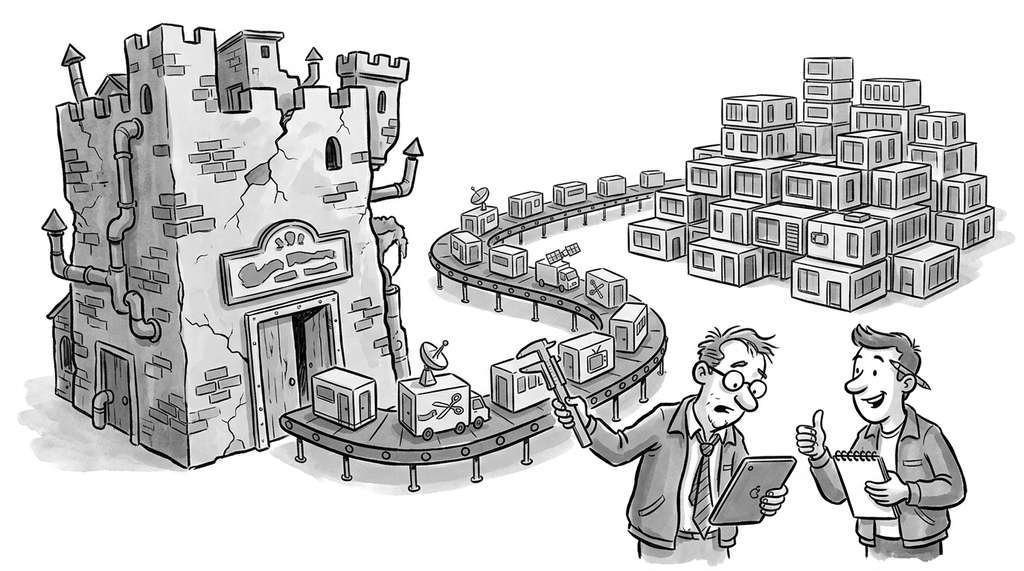
6. Weighted Selection from the Frontier

When stakeholders do express preferences as weights, we can select the frontier candidate closest to their ideal point. The ideal point is the vector of best possible scores across all attributes; no real architecture achieves it, but we can find the frontier candidate that minimizes weighted Euclidean distance (the square root of the sum of squared per-attribute gaps to the ideal, each scaled by that attribute's importance weight) to it.

def select_from_frontier(
    frontier_indices: list[int],
    metrics: list[dict[str, float]],
    weights: dict[str, float],
) -> int:
    """Select the best candidate from the Pareto frontier using weighted
    distance to the ideal point.

    Args:
        frontier_indices: Indices of frontier candidates.
        metrics: All candidate metrics.
        weights: Stakeholder preference weights per attribute.

    Returns:
        Index of the selected candidate.
    """
    keys = sorted(metrics[0].keys())

    # Ideal point: best score for each attribute across ALL candidates
    all_scores = np.array([[m[k] for k in keys] for m in metrics])
    ideal = np.max(all_scores, axis=0)

    # Weight vector (aligned with keys)
    w = np.array([weights.get(k, 1.0) for k in keys])
    w = w / w.sum()  # normalize

    # Find frontier candidate closest to ideal (weighted Euclidean)
    best_idx = None
    best_dist = float("inf")
    for idx in frontier_indices:
        scores = np.array([metrics[idx][k] for k in keys])
        dist = np.sqrt(np.sum(w * (ideal - scores) ** 2))
        if dist < best_dist:
            best_dist = dist
            best_idx = idx

    return best_idx


# Stakeholder weights: scalability and deployability matter most
stakeholder_weights = {
    "maintainability": 0.2,
    "performance": 0.2,
    "scalability": 0.35,
    "deployability": 0.25,
}

selected = select_from_frontier(
    frontier_indices, style_metrics, stakeholder_weights
)
print(f"Selected: {style_names[selected]}")
# Output: Selected: Microservices

When stakeholders weight scalability and deployability highest, microservices win. Shift the weights toward performance and maintainability, and the hexagonal style wins instead. This sensitivity analysis (systematically varying the weights to observe whether the selected candidate changes) shows stakeholders how robust their choice is to priority shifts.

7. The Complete Generation Pipeline

The generation, conversion, scoring, and selection stages wire together into a single callable function.

Putting it all together, the architecture generation pipeline follows five steps. Figure 14.2 illustrates the flow from validated requirements through LLM generation, graph conversion, Pareto analysis, and weighted selection.

1. Input: Validated requirements from Chapter 13 and stakeholder quality-attribute weights.
2. Generate: Use the LLM to produce 3 to 5 candidate architectures as structured ArchitectureProposal objects.
3. Convert: Transform each candidate into a NetworkX graph and compute quality metrics.
4. Analyze: Compute the Pareto frontier and select the optimal candidate using stakeholder weights.
5. Visualize: Generate Mermaid diagrams and metric comparison tables for stakeholder review.

def run_architecture_discovery(
    requirements: list[str],
    quality_weights: dict[str, float],
    num_candidates: int = 3,
) -> dict:
    """Run the full architecture discovery pipeline.

    Returns a dictionary containing all candidates, their metrics,
    the Pareto frontier, the selected candidate, and Mermaid diagrams.
    """
    # Step 1: Generate candidates via LLM
    proposal = generate_architecture_candidates(
        requirements, quality_weights, num_candidates
    )

    # Step 2: Convert to graphs and compute metrics
    graphs = []
    all_metrics = []
    mermaid_diagrams = []

    for candidate in proposal.candidates:
        graph = candidate_to_graph(candidate)
        metrics = compute_architecture_metrics(graph)
        mermaid = graph_to_mermaid(graph, candidate.name)

        graphs.append(graph)
        all_metrics.append(metrics)
        mermaid_diagrams.append(mermaid)

    # Step 3: Compute Pareto frontier
    candidate_names = [c.name for c in proposal.candidates]
    frontier = compute_pareto_frontier(
        candidate_names, all_metrics, maximize=True
    )

    # Step 4: Select best from frontier
    selected_idx = select_from_frontier(
        frontier, all_metrics, quality_weights
    )

    return {
        "system_name": proposal.system_name,
        "candidates": [
            {
                "name": c.name,
                "style": c.style.value,
                "rationale": c.rationale,
                "tradeoffs": c.tradeoffs,
                "metrics": all_metrics[i],
                "mermaid": mermaid_diagrams[i],
                "on_frontier": i in frontier,
            }
            for i, c in enumerate(proposal.candidates)
        ],
        "frontier_indices": frontier,
        "selected_index": selected_idx,
        "selected_name": candidate_names[selected_idx],
    }

Exercises

1. Conceptual: Explain why generating architectures with a single LLM call might produce less diverse candidates than generating them with multiple independent calls (one per style). What prompt engineering techniques from Chapter 10 could improve diversity within a single call?
2. Coding: Extend the graph_to_mermaid function to generate Structurizr DSL instead of Mermaid. The Structurizr DSL uses a workspace block containing model (defining people, software systems, containers, and components) and views (defining which diagrams to render). Generate a Container diagram for any architecture graph.
3. Analysis: Run the run_architecture_discovery pipeline three times with the same requirements but different quality weights. How stable is the Pareto frontier across runs? How sensitive is the selected candidate to the weights? Document your findings as a sensitivity analysis table.