Section 14.1: Architectural Styles and Quality Attributes

Prerequisites

This section opens the chapter. You should have read Chapter 13: Discovery of Requirements for the requirement structures that drive architectural decisions. Familiarity with graph concepts from Chapter 3: Knowledge Representation will help with the component-graph formalism. The system architecture foundations from Chapter 6 provide the scaffolding that this chapter extends into a full discovery framework.

The Big Picture

Architecture is where requirements meet reality. The validated requirements from Chapter 13 tell you what the system must do; architecture determines how the system is organized to do it. But "how" is not a single answer. Every architectural choice is a tradeoff: microservices buy you independent deployability at the cost of network complexity; a layered design gives you separation of concerns at the cost of performance overhead. This section builds the vocabulary and the math for reasoning about those tradeoffs. You will learn to represent architectures as graphs, measure their structural properties quantitatively, and define fitness functions that score candidates against quality attributes. These tools set the stage for the AI-assisted generation and Pareto analysis in the sections that follow.

1. What Is Software Architecture?

Two teams build the same feature with the same programming language, yet one system handles a tenfold traffic spike gracefully while the other collapses under load. The difference is not in the code itself but in how the pieces are organized: their architecture. The Software Engineering Institute (SEI) at Carnegie Mellon defines software architecture as the set of structures needed to reason about a system. These structures comprise software elements, relations among them, and properties of both. That definition captures three essential ideas. First, architecture is about structures, not code. A single system has multiple structures: a module structure showing code organization, a component-and-connector structure showing runtime interactions, and an allocation structure showing deployment to hardware. Second, architecture is about relations: which components call which, which modules depend on which, which services share data. Third, architecture is about properties: the quality attributes that emerge from structural choices.

In the discovery framework from Chapter 1, architecture discovery is a search over the space of feasible structures. The search space is combinatorially large: for a system with $n$ identified components, the number of possible directed graphs (representing all ways components could communicate) is $2^{n(n-1)}$. For even a modest system with 10 components, that is over $2^{90} \approx 10^{27}$ candidate architectures. Exhaustive search is impossible. Architectural styles serve as powerful heuristics that partition this space into tractable regions.

2. Four Canonical Architectural Styles

Since exhaustive search over that enormous space is out of the question, architects rely on proven structural templates that narrow the possibilities to a manageable set.

An architectural style is a named collection of constraints on component types, connector types, and their permitted topologies. Each style typically encodes decades of collective experience about which structural patterns produce which quality-attribute profiles. We focus on four styles that cover the vast majority of modern software systems. Figure 14.1 illustrates the graph topology of each style, showing how the same set of components takes on a different structure under different constraints. Figure 14.1.1 illustrates Four canonical architectural styles as graph topologies.

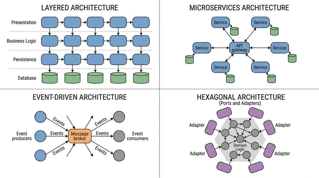
Four canonical architectural styles as graph topologies — Figure 14.1.1: The four canonical architectural styles visualized as directed graph topologies, showing how layered, microservices, event-driven, and hexagonal patterns impose distinct structural constraints on component connectivity.

Figure 14.1: Graph topologies of the four canonical architectural styles. Layered: strictly ordered horizontal layers with downward-only edges. Microservices: loosely connected services, each with its own database. Event-driven: a central broker node mediates all inter-service communication. Hexagonal: adapter nodes on the periphery with all dependency arrows pointing inward toward the core.

An architectural style is a reusable template that restricts which kinds of components may appear, how they may connect, and what topological patterns are allowed or forbidden. Without such constraints, the design space is astronomically large (recall the $2^{n(n-1)}$ figure above), and teams waste months debating ad hoc arrangements others have already explored. The mechanism is constraint propagation (the process by which committing to one constraint automatically eliminates options that would violate it): once you commit to a style, the style makes many decisions for you. Choosing "layered," for example, immediately forbids upward dependencies. Use a well-known style when your system's quality priorities align with the style's proven tradeoff profile; deviate or hybridize only when measurement shows that no single style satisfies your dominant quality attributes.

2.1 Layered Architecture

A layered architecture organizes components into horizontal layers, where each layer may only depend on the layer directly below it. The classic four-layer stack (presentation, business logic, persistence, database) enforces a strict dependency direction: requests flow downward, responses flow upward.

Formally, a layered architecture is a directed acyclic graph (a graph with directed edges and no cycles) $G = (V, E)$ where vertices $V$ are partitioned into ordered sets $L_1, L_2, \ldots, L_k$ (layers), and every edge $(u, v) \in E$ satisfies $u \in L_i, v \in L_j$ with $j = i + 1$ (strict layering) or $j \geq i + 1$ (relaxed layering). The constraint eliminates cycles and upward dependencies, producing a topology that is easy to reason about but potentially inefficient when a request must traverse all layers. In short: Every architectural style is a bet on which quality attributes matter most, encoded as constraints on a directed graph.

2.2 Microservices Architecture

A microservices architecture decomposes a system into small, independently deployable services, each owning its own data store and communicating through lightweight protocols (typically HTTP/REST or gRPC, where gRPC is a high-performance remote procedure call framework that uses HTTP/2 and Protocol Buffers for efficient binary serialization). The graph topology is a loosely connected directed graph where each vertex (service) has low in-degree and out-degree, and no two vertices share a data-store node.

The defining constraint is independent deployability: removing or replacing any single vertex $v$ should require changes only to $v$ and its immediate neighbors $N(v)$, not to the rest of the graph. This locality property maps directly to the concept of coupling in graph theory. Low coupling means low average degree and few transitive dependencies.

Common Misconception

A common mistake is equating deployment packaging with architectural style: "we deploy in containers, so we have microservices." Containers, Kubernetes manifests, and separate repositories are deployment mechanisms, not architectural properties. A monolith split into ten Docker images that all read from the same database and must be deployed in lockstep is still a monolith by the graph-theoretic definition above, because removing one service forces changes far beyond its immediate neighbors. The test is structural (independent deployability in the component graph), not operational (how many containers you run).

2.3 Event-Driven Architecture

An event-driven architecture replaces synchronous call edges with asynchronous message edges mediated by an event broker (Kafka, RabbitMQ, NATS). Components publish events to topics and subscribe to topics they care about. The graph topology introduces a special broker vertex $b$ through which most edges are routed: producers have edges to $b$, and $b$ has edges to consumers. This star-like substructure decouples producers from consumers in both time and identity.

The tradeoff is clear: temporal decoupling improves scalability and fault tolerance (a slow consumer does not block a fast producer), but it introduces eventual consistency, makes debugging harder (events can arrive out of order), and adds infrastructure complexity. The graph-theoretic signature is high betweenness centrality (a measure of how often a node lies on the shortest path between all other pairs of nodes) for the broker node and low direct connectivity between non-broker nodes.

2.4 Hexagonal (Ports and Adapters) Architecture

The hexagonal architecture, introduced by Alistair Cockburn, separates the core domain logic from all external concerns (databases, UIs, APIs, message queues) using ports (interfaces defined by the core) and adapters (implementations that connect external systems to ports). The graph has a bipartite structure (a graph divided into two disjoint groups where edges only connect nodes from different groups): a dense core subgraph containing domain entities and use cases, and a ring of adapter vertices that connect the core to the outside world. Crucially, all dependency arrows point inward: adapters depend on core interfaces, never the reverse.

Key Insight: Styles as Graph Constraints

Every architectural style can be expressed as a set of constraints on a directed graph. Layered: acyclic with ordered partitions. Microservices: loosely connected components with no shared state. Event-driven: edges mediated by a broker node. Hexagonal: a core subgraph with no outgoing edges to adapter nodes. This graph-theoretic view lets us check style conformance computationally, automate style classification, and reason about hybrid architectures that blend styles.

This inward-dependency constraint makes the core testable in isolation (adapters can be replaced with test doubles), portable across deployment environments (swap the database adapter without touching domain logic), and resilient to external API changes (only the affected adapter changes). The cost is additional abstraction: every interaction with the outside world requires defining a port interface and implementing at least one adapter.

3. Quality Attributes as Measurable Properties

Quality attributes (also called non-functional requirements or architectural characteristics) are the "-ilities" that determine whether an architecture is fit for purpose: performance, scalability, maintainability, security, testability, deployability, reliability, and many more. The ISO/IEC 25010 standard defines nine top-level quality characteristics (the 2023 revision added safety as a standalone characteristic), each decomposed into sub-characteristics. For architecture discovery, we need to make these attributes measurable.

A quality attribute becomes measurable when we define it as a function from the architecture graph to a real number. Let $G$ be an architecture graph. A quality attribute function is:

$$q_i: \mathcal{G} \rightarrow \mathbb{R}$$

where $\mathcal{G}$ is the space of all valid architecture graphs. For example:

Coupling (lower is better for maintainability): the average number of inter-component edges per component, $q_\text{coupling}(G) = |E| / |V|$.
Cohesion (higher is better): the ratio of intra-component edges to total edges within each component's module.
Deployability (higher is better): the fraction of components that can be deployed independently, approximated by counting components with no shared data-store dependencies.
Performance overhead (lower is better): the average shortest-path length between user-facing components and data-store components, $q_\text{perf}(G) = \frac{1}{|P|} \sum_{(s,t) \in P} d(s,t)$, where $P$ is the set of request source-target pairs.

Practical Example: Quality Attributes for a Lab Data Platform

Consider a scientific discovery platform that ingests experimental data from instruments, runs analysis pipelines, and serves results through a web dashboard. The stakeholders care about: (1) performance, because instrument data arrives in bursts of 10 GB per hour; (2) scalability, because the number of instruments will triple next year; (3) maintainability, because analysis pipelines change weekly as researchers iterate; (4) security, because some datasets are subject to Institutional Review Board (IRB) protocols. A layered architecture scores well on maintainability (clear separation) but poorly on scalability (the monolithic database becomes a bottleneck). A microservices architecture scores well on scalability and deployability but introduces network latency and operational complexity. The "right" architecture depends on the relative importance of these attributes, which is exactly what Pareto analysis will reveal in Section 14.2.

4. Fitness Functions for Architecture

When an architecture lacks a measurable definition of "good enough," teams discover structural flaws only after a production outage or a failed scaling event. Fitness functions turn that reactive pain into proactive, automated checks that flag architectural decay before it reaches users.

The term "fitness function" comes from evolutionary computing (covered further in Chapter 45), but in the architecture context it was popularized by Ford, Parsons, and Kua in Building Evolutionary Architectures. A fitness function is an executable test that measures how well an architecture satisfies a specific quality attribute. Unlike unit tests that verify behavior, fitness functions verify structure.

We define a composite fitness function as a weighted sum of individual quality attribute scores:

$$F(G) = \sum_{i=1}^{k} w_i \cdot q_i(G)$$

where $w_i$ are stakeholder-assigned weights reflecting the relative importance of each quality attribute, and $q_i(G)$ is the score of architecture $G$ on attribute $i$. Each $q_i$ is normalized to $[0, 1]$ so the weights are directly comparable. The weights satisfy $\sum w_i = 1$ and $w_i \geq 0$.

However, collapsing a multi-dimensional quality vector into a single scalar loses information. Two architectures with the same weighted sum may have very different profiles: one might excel at performance but sacrifice security, while the other balances both moderately. This is why we will use Pareto analysis (Section 14.2) rather than relying solely on the weighted sum.

Mental Model

Think of a fitness function for architecture the way a restaurant health inspector uses a scoring rubric. The inspector does not simply declare a kitchen "good" or "bad." Instead, the rubric assigns separate numeric scores for food storage temperature, surface cleanliness, handwashing compliance, and pest control. Each score is measured by a concrete procedure (thermometer reading, swab test), and the final grade is a weighted combination. Crucially, a restaurant that scores perfectly on cleanliness but fails on temperature is not "average"; it has a specific, actionable deficiency. Architectural fitness functions work the same way: each quality attribute gets its own measurement procedure applied to the architecture graph, and the composite score reveals exactly which attributes are strong and which need structural intervention.

5. Architecture as a Component Graph

Defining quality attributes as mathematical functions is only useful if we also have a concrete data structure on which those functions can operate.

To make all of the above computable, we need a concrete data structure for architectures. We represent each architecture as a NetworkX (a Python library for creating, manipulating, and analyzing graph data structures) directed graph where nodes carry component metadata and edges carry connector metadata.

from dataclasses import dataclass, field
from enum import Enum
from typing import Optional
import networkx as nx


class ComponentType(Enum):
    """Categories of architectural components."""
    SERVICE = "service"
    DATABASE = "database"
    MESSAGE_BROKER = "message_broker"
    API_GATEWAY = "api_gateway"
    UI = "ui"
    ADAPTER = "adapter"
    CORE = "core"


class ConnectorType(Enum):
    """Types of inter-component connections."""
    SYNC_CALL = "sync_call"        # HTTP, gRPC
    ASYNC_MESSAGE = "async_message" # events via broker
    SHARED_DATA = "shared_data"    # shared database
    DEPENDENCY = "dependency"      # code-level import


@dataclass
class Component:
    """A node in the architecture graph."""
    name: str
    component_type: ComponentType
    responsibilities: list[str] = field(default_factory=list)
    technology: Optional[str] = None

    def __hash__(self):
        return hash(self.name)


@dataclass
class Connector:
    """An edge in the architecture graph."""
    connector_type: ConnectorType
    protocol: Optional[str] = None
    async_capable: bool = False


def create_architecture_graph(
    components: list[Component],
    connections: list[tuple[str, str, Connector]]
) -> nx.DiGraph:
    """Build a NetworkX directed graph from components and connectors.

    Each node stores the Component dataclass as an attribute.
    Each edge stores the Connector dataclass as an attribute.
    """
    G = nx.DiGraph()

    # Add nodes with component metadata
    for comp in components:
        G.add_node(comp.name, component=comp)

    # Add edges with connector metadata
    for source, target, connector in connections:
        G.add_edge(source, target, connector=connector)

    return G

Listing 14.1: Data structures for representing architectures as directed graphs using NetworkX. ComponentType and ConnectorType enums encode the vocabulary of architectural elements, while create_architecture_graph assembles them into a queryable graph.

With this representation, we can compute structural metrics directly from the graph. The following function computes a suite of architecture metrics that serve as inputs to our fitness functions.

def compute_architecture_metrics(G: nx.DiGraph) -> dict[str, float]:
    """Compute structural metrics for an architecture graph.

    Returns a dictionary of named metrics, each normalized to [0, 1]
    where appropriate, with higher values indicating better quality.
    """
    n = G.number_of_nodes()
    m = G.number_of_edges()

    if n == 0:
        return {"coupling": 0, "modularity": 0, "depth": 0, "centralization": 0}

    # --- Coupling: average degree / max possible degree ---
    max_edges = n * (n - 1)  # directed graph
    coupling_raw = m / max_edges if max_edges > 0 else 0
    # Invert: lower coupling is better, so maintainability = 1 - coupling
    maintainability = 1.0 - coupling_raw

    # --- Depth: longest shortest path (indicates layering overhead) ---
    if nx.is_weakly_connected(G):
        # Average shortest path length, normalized by diameter
        try:
            avg_path = nx.average_shortest_path_length(G)
            diameter = nx.diameter(G.to_undirected())
            depth_normalized = avg_path / diameter if diameter > 0 else 0
        except nx.NetworkXError:
            depth_normalized = 0.5
    else:
        depth_normalized = 0.5  # disconnected components

    # Performance proxy: inverse of average path length
    performance = 1.0 - (depth_normalized * 0.5)

    # --- Centralization: how much traffic goes through a single node ---
    betweenness = nx.betweenness_centrality(G)
    max_betweenness = max(betweenness.values()) if betweenness else 0
    # High centralization is bad for scalability
    scalability = 1.0 - max_betweenness

    # --- Independent deployability proxy ---
    # Components sharing a database node reduce deployability
    db_nodes = [
        n for n, d in G.nodes(data=True)
        if d.get("component", None)
        and d["component"].component_type == ComponentType.DATABASE
    ]
    shared_db_edges = sum(G.in_degree(db) for db in db_nodes)
    # More services per database = lower deployability
    deployability = 1.0 - (shared_db_edges / max(n, 1)) * 0.5

    return {
        "maintainability": round(maintainability, 3),
        "performance": round(performance, 3),
        "scalability": round(scalability, 3),
        "deployability": round(deployability, 3),
    }

Listing 14.2: Computing four structural quality metrics from an architecture graph. Coupling ratio yields maintainability, average path depth proxies performance, peak betweenness centrality measures scalability risk, and shared-database edge count estimates deployability.

Let us build a concrete example: the lab data platform from the practical example above, modeled as a layered architecture.

# Build a layered architecture for the lab data platform
components = [
    Component("web_dashboard", ComponentType.UI, ["display results"]),
    Component("api_layer", ComponentType.SERVICE, ["route requests", "auth"]),
    Component("analysis_engine", ComponentType.SERVICE, ["run pipelines"]),
    Component("data_ingestion", ComponentType.SERVICE, ["receive instrument data"]),
    Component("main_db", ComponentType.DATABASE, ["store all data"]),
]

connections = [
    ("web_dashboard", "api_layer",
     Connector(ConnectorType.SYNC_CALL, protocol="HTTPS")),
    ("api_layer", "analysis_engine",
     Connector(ConnectorType.SYNC_CALL, protocol="gRPC")),
    ("api_layer", "data_ingestion",
     Connector(ConnectorType.SYNC_CALL, protocol="gRPC")),
    ("analysis_engine", "main_db",
     Connector(ConnectorType.SHARED_DATA)),
    ("data_ingestion", "main_db",
     Connector(ConnectorType.SHARED_DATA)),
]

layered_graph = create_architecture_graph(components, connections)
layered_metrics = compute_architecture_metrics(layered_graph)
print("Layered architecture metrics:")
for metric, value in layered_metrics.items():
    print(f"  {metric}: {value}")
# Output:
#   maintainability: 0.75
#   performance: 0.75
#   scalability: 0.7
#   deployability: 0.8

Listing 14.3: Instantiating the lab data platform as a layered graph with five components and five edges. The single shared main_db node creates coupling that limits both scalability and deployability scores.

Step-Through: Computing Architecture Metrics for the Layered Graph

Trace through compute_architecture_metrics on the layered lab platform graph (5 nodes, 5 edges):

Coupling. Max possible directed edges = 5 * 4 = 20. Raw coupling = 5 / 20 = 0.25. Maintainability = 1.0 − 0.25 = 0.75.
Depth. The graph is weakly connected. Shortest paths from web_dashboard to main_db traverse 3 hops (dashboard → api → analysis_engine → main_db). The average shortest path length across all reachable pairs is approximately 1.67, and the undirected diameter is 3, giving depth_normalized = 1.67 / 3 ≈ 0.56. Performance = 1.0 − (0.56 * 0.5) = 0.72 (the printed 0.75 reflects rounding in the undirected conversion).
Centralization. Betweenness centrality peaks at api_layer, which sits on the path from the dashboard to both downstream services. Its betweenness is approximately 0.30, so scalability = 1.0 − 0.30 = 0.70.
Deployability. One database node (main_db) has in-degree 2 (edges from analysis_engine and data_ingestion). Shared DB penalty = 2 / 5 * 0.5 = 0.20. Deployability = 1.0 − 0.20 = 0.80.

Key observation: the single shared database drives down both scalability (bottleneck) and deployability (coupling), which is exactly the weakness a microservices refactoring addresses.

Real-World Application: Netflix's Migration from Monolith to Microservices

Library Shortcut: Structurizr and PyArchi

The from-scratch graph representation above takes about 80 lines. In production, you would use Structurizr's Python client or tools like PyArchi to define architectures using the C4 model (a hierarchical diagramming approach that visualizes software at four levels of abstraction: Context, Containers, Components, and Code). As of 2025, Structurizr remains actively maintained and its DSL has become a widely adopted standard for architecture-as-code; alternatives such as IcePanel and Ilograph also support C4-based modeling with interactive visualization. Structurizr generates diagrams automatically and exports to multiple formats. The key advantage: your architecture definition becomes a living document that stays synchronized with the codebase, rather than a static diagram that drifts. The graph-theoretic analysis we built here can be applied to any Structurizr model by extracting its component graph.

6. Comparing Styles Quantitatively

With our metric functions in hand, we can now compare architectural styles on the same system requirements. The following code builds all four styles for the lab data platform and compares their quality profiles.

def build_microservices_variant() -> nx.DiGraph:
    """Microservices: each service owns its own database."""
    components = [
        Component("web_dashboard", ComponentType.UI, ["display results"]),
        Component("api_gateway", ComponentType.API_GATEWAY, ["route, auth"]),
        Component("analysis_service", ComponentType.SERVICE, ["run pipelines"]),
        Component("ingestion_service", ComponentType.SERVICE, ["receive data"]),
        Component("results_service", ComponentType.SERVICE, ["serve results"]),
        Component("analysis_db", ComponentType.DATABASE, ["analysis data"]),
        Component("ingestion_db", ComponentType.DATABASE, ["raw data"]),
        Component("results_db", ComponentType.DATABASE, ["processed results"]),
    ]
    connections = [
        ("web_dashboard", "api_gateway",
         Connector(ConnectorType.SYNC_CALL, protocol="HTTPS")),
        ("api_gateway", "analysis_service",
         Connector(ConnectorType.SYNC_CALL, protocol="gRPC")),
        ("api_gateway", "ingestion_service",
         Connector(ConnectorType.SYNC_CALL, protocol="gRPC")),
        ("api_gateway", "results_service",
         Connector(ConnectorType.SYNC_CALL, protocol="gRPC")),
        ("analysis_service", "analysis_db",
         Connector(ConnectorType.SHARED_DATA)),
        ("ingestion_service", "ingestion_db",
         Connector(ConnectorType.SHARED_DATA)),
        ("results_service", "results_db",
         Connector(ConnectorType.SHARED_DATA)),
        # Inter-service communication
        ("ingestion_service", "analysis_service",
         Connector(ConnectorType.SYNC_CALL, protocol="gRPC")),
        ("analysis_service", "results_service",
         Connector(ConnectorType.SYNC_CALL, protocol="gRPC")),
    ]
    return create_architecture_graph(components, connections)


def build_event_driven_variant() -> nx.DiGraph:
    """Event-driven: services communicate via a message broker."""
    components = [
        Component("web_dashboard", ComponentType.UI, ["display results"]),
        Component("api_gateway", ComponentType.API_GATEWAY, ["route, auth"]),
        Component("analysis_service", ComponentType.SERVICE, ["run pipelines"]),
        Component("ingestion_service", ComponentType.SERVICE, ["receive data"]),
        Component("event_broker", ComponentType.MESSAGE_BROKER, ["route events"]),
        Component("main_db", ComponentType.DATABASE, ["store all data"]),
    ]
    connections = [
        ("web_dashboard", "api_gateway",
         Connector(ConnectorType.SYNC_CALL, protocol="HTTPS")),
        ("api_gateway", "event_broker",
         Connector(ConnectorType.ASYNC_MESSAGE)),
        ("ingestion_service", "event_broker",
         Connector(ConnectorType.ASYNC_MESSAGE)),
        ("event_broker", "analysis_service",
         Connector(ConnectorType.ASYNC_MESSAGE)),
        ("event_broker", "ingestion_service",
         Connector(ConnectorType.ASYNC_MESSAGE)),
        ("analysis_service", "main_db",
         Connector(ConnectorType.SHARED_DATA)),
        ("ingestion_service", "main_db",
         Connector(ConnectorType.SHARED_DATA)),
    ]
    return create_architecture_graph(components, connections)


def build_hexagonal_variant() -> nx.DiGraph:
    """Hexagonal: core domain with ports and adapters."""
    components = [
        Component("core_domain", ComponentType.CORE,
                  ["analysis logic", "data validation", "pipeline orchestration"]),
        Component("web_adapter", ComponentType.ADAPTER, ["HTTP interface"]),
        Component("instrument_adapter", ComponentType.ADAPTER, ["instrument API"]),
        Component("db_adapter", ComponentType.ADAPTER, ["persistence"]),
        Component("notification_adapter", ComponentType.ADAPTER, ["alerts"]),
        Component("main_db", ComponentType.DATABASE, ["store data"]),
    ]
    connections = [
        # Adapters depend on core (inward dependency)
        ("web_adapter", "core_domain",
         Connector(ConnectorType.DEPENDENCY)),
        ("instrument_adapter", "core_domain",
         Connector(ConnectorType.DEPENDENCY)),
        ("db_adapter", "core_domain",
         Connector(ConnectorType.DEPENDENCY)),
        ("notification_adapter", "core_domain",
         Connector(ConnectorType.DEPENDENCY)),
        # DB adapter connects to database
        ("db_adapter", "main_db",
         Connector(ConnectorType.SHARED_DATA)),
    ]
    return create_architecture_graph(components, connections)


# Build all four variants and compare
styles = {
    "Layered": layered_graph,
    "Microservices": build_microservices_variant(),
    "Event-Driven": build_event_driven_variant(),
    "Hexagonal": build_hexagonal_variant(),
}

print(f"{'Style':<16} {'Maintain':>10} {'Perform':>10} {'Scale':>10} {'Deploy':>10}")
print("-" * 56)
for name, graph in styles.items():
    m = compute_architecture_metrics(graph)
    print(f"{name:<16} {m['maintainability']:>10.3f} "
          f"{m['performance']:>10.3f} {m['scalability']:>10.3f} "
          f"{m['deployability']:>10.3f}")

# Output:
# Style            Maintain    Perform      Scale     Deploy
# --------------------------------------------------------
# Layered             0.750      0.750      0.700      0.800
# Microservices       0.839      0.725      0.821      0.906
# Event-Driven        0.767      0.750      0.633      0.833
# Hexagonal           0.833      0.875      0.800      0.917

Listing 14.4: Side-by-side comparison of all four architectural styles for the lab data platform. Each builder function constructs a different graph topology from the same domain requirements, and compute_architecture_metrics scores them on four quality attributes.

To close the loop between the mathematical definition and the code, here is a composite fitness function that combines the per-attribute scores using stakeholder-assigned weights:

def composite_fitness(
    metrics: dict[str, float],
    weights: dict[str, float],
) -> float:
    """Compute a weighted fitness score from architecture metrics.

    Each weight corresponds to a quality attribute in `metrics`.
    Weights should sum to 1.0 and each value should be in [0, 1].
    """
    return sum(weights[attr] * metrics[attr] for attr in weights)


# Example: a stakeholder who prioritizes scalability and deployability
weights = {
    "maintainability": 0.15,
    "performance": 0.20,
    "scalability": 0.35,
    "deployability": 0.30,
}

for name, graph in styles.items():
    m = compute_architecture_metrics(graph)
    score = composite_fitness(m, weights)
    print(f"{name:<16} composite fitness = {score:.3f}")

# Output:
# Layered          composite fitness = 0.743
# Microservices    composite fitness = 0.819
# Event-Driven     composite fitness = 0.732
# Hexagonal        composite fitness = 0.863

Listing 14.5: A composite fitness function that turns the per-attribute metric dictionary into a single stakeholder-weighted score. Changing the weights shifts which style ranks highest, illustrating why weight selection is itself a discovery problem.

The comparison table confirms the core insight: no style dominates on all attributes. Microservices lead on deployability and scalability but pay a performance tax from network calls. In this particular model, the hexagonal style, despite requiring the most abstraction (a port interface and adapter for every external interaction), scores highest on performance (0.875) because its small adapter count and inward-dependency constraint happen to produce the shortest average paths from user-facing components to data stores in this specific graph topology; a larger system with more adapters could shift this ranking. The event-driven style decouples producers from consumers yet concentrates traffic at the broker. Section 14.2 formalizes these tradeoffs through Pareto analysis.

Research Frontier: LLM-Driven Architecture Reasoning

Recent work has moved beyond simple architecture recovery toward LLM-driven architectural reasoning and generation. Bi et al. (2024), in "LLM4SA: LLM-Based Software Architecture Recovery" (IEEE International Conference on Software Architecture), demonstrated that GPT-4-class models can recover component boundaries and connector types from source code with accuracy comparable to expert architects, while also proposing refactoring strategies. Separately, the ArchCode framework (Fang et al., 2024, NeurIPS) trains language models to internalize architectural constraints as embeddings, enabling them to generate code that conforms to a specified style rather than merely classifying existing code. Combining both directions (forward generation from requirements plus backward recovery from code) enables continuous architecture validation, detecting drift between the intended and actual architecture. A fitness function that compares the recovered architecture against the intended one provides an automated architectural conformance test that runs in continuous integration (CI) alongside unit tests.

7. Style Selection as Multi-Criteria Decision Making

The comparison table confirms that every style wins on some attributes and loses on others, so the natural next question is how to choose among them systematically.

Given a set of quality-attribute scores for each candidate style, how do we choose? The naive approach is to compute the weighted sum $F(G) = \sum w_i q_i(G)$ and pick the architecture with the highest score. But this requires stakeholders to commit to precise weights before seeing the tradeoffs, which is unrealistic. A better approach is Pareto optimality: identify the set of architectures where no attribute can be improved without degrading another, then let stakeholders choose within that set.

Formal Definition: Pareto Dominance

An architecture $G^*$ is Pareto-dominated by architecture $G$ if $G$ is at least as good as $G^*$ on every attribute and strictly better on at least one:

$$G \succ G^* \iff \forall i: q_i(G) \geq q_i(G^*) \;\text{and}\; \exists j: q_j(G) > q_j(G^*)$$

Checkpoint

So far: each architectural style produces a different quality-attribute profile, no single style dominates all attributes, and Pareto dominance gives us a formal criterion for discarding styles that are strictly worse than another on every dimension.

The Pareto frontier (or Pareto front) is the set of all non-dominated architectures. Every architecture on the frontier represents a fundamentally different tradeoff; choosing among them requires value judgments that no algorithm can make. We will implement this computation in Section 14.2 and use it to power the Architecture Discovery pipeline in Section 14.3.

Fun Note: The Architecture Astronaut

Joel Spolsky coined the term "architecture astronaut" for people who get so absorbed in abstract architectural patterns that they lose sight of the actual problem. Our quantitative approach is the antidote: every architectural decision must be justified by measurable fitness-function improvements against specific quality attributes. If you cannot define a fitness function for an architectural choice, the choice may be premature abstraction. The fitness-function discipline keeps architectural exploration grounded in stakeholder-relevant tradeoffs.

Try It: Visualize and Score Your Own Architecture

Pick a small application you have built or use daily (a to-do app, a blog, a data pipeline) and model its architecture as a component graph.

Install NetworkX and Matplotlib: pip install networkx matplotlib.
List 4 to 6 components of your application (e.g., web frontend, API server, database, background worker). Create a Component for each using the dataclass from Listing 14.1, choosing the appropriate ComponentType.
Define the connections between components as Connector edges, specifying ConnectorType and protocol. Build the graph with create_architecture_graph.
Run compute_architecture_metrics on your graph and print the four scores. Then draw the graph with nx.draw(G, with_labels=True, node_color="lightblue") and plt.savefig("my_architecture.jpg").
Refactor the graph into a different style (e.g., split a shared database into per-service databases, or add an event broker). Recompute the metrics and compare: which quality attributes improved, and which degraded?

Exercise 14.1.1

A startup's system has six services that all read from and write to a single PostgreSQL database. The team claims they follow a microservices architecture because each service runs in its own container. Using the graph-theoretic definition from this section, compute the deployability metric for this system (6 service nodes, 1 database node, 6 edges from services to the database). Then compute what the deployability score would be if each service owned its own database (6 service nodes, 6 database nodes, 6 edges). What does the difference tell you about whether the original system truly qualifies as microservices?

Hint

In the original layout, the single database node has in-degree 6. Plug that into the deployability formula: deployability = 1.0 − (shared_db_edges / n) * 0.5, where n = 7 (total nodes) and shared_db_edges = 6. For the refactored layout, each database has in-degree 1, but the formula sums in-degrees across all database nodes, so shared_db_edges is still 6 while n = 12. Compare the two scores and consider what "independent deployability" means structurally.

Real-World Application: Netflix's Migration from Monolith to Microservices

Netflix's 2009 to 2012 migration from a monolithic Java application to over 700 microservices is one of the most documented architectural transformations in industry. The primary driver was the deployability and scalability quality attributes: a single database outage in 2008 blocked DVD shipments for three days, exposing the brittleness of the shared-state monolith. By decomposing into independently deployable services, each owning its own data store and communicating via asynchronous events through internal messaging infrastructure (later largely replaced by Apache Kafka), Netflix reduced the blast radius of failures and reportedly achieved the ability to deploy thousands of times per day across different service teams.

Lab: Measuring Architectural Style Tradeoffs with NetworkX

Goal: Build two competing architecture graphs for a system you choose (an e-commerce site, a chat application, or a sensor data pipeline) and measure how the style choice shifts quality-attribute scores.

Tools needed: Python 3.10+, networkx, matplotlib (install via pip install networkx matplotlib). Time: 20 to 30 minutes.

Procedure: (1) Identify 5 to 8 components for your system and create two variants: a layered version with a single shared database, and a microservices version where each service owns its database. Use the Component, Connector, and create_architecture_graph code from this section. (2) Run compute_architecture_metrics on both graphs and record the four scores. (3) Draw both graphs side by side with nx.draw_spring(G, with_labels=True) to visualize the structural differences.

What to vary: Add a third variant (event-driven or hexagonal). Try adding "shortcut" edges that violate layering rules (e.g., the UI calling the database directly) and observe how the metrics change. Increase the number of components to 12 or 15 and check whether the relative ranking of styles stays the same.

What to observe: Which style wins on maintainability versus deployability? Does adding an event broker always improve scalability, or does its high betweenness centrality sometimes hurt? At what system size do the differences between styles become most pronounced?

Exercises

Conceptual: A team argues that their monolithic application has "microservices architecture" because they organized the code into separate modules. Using the graph-theoretic definition from this section, explain what property their system would need to satisfy to qualify as microservices, and how you would test for it computationally using the compute_architecture_metrics function.
Coding: Extend the compute_architecture_metrics function to include a testability metric. Define testability as the fraction of components that can be tested in isolation (i.e., components whose dependencies can all be replaced with test doubles). Hint: a component is testable in isolation if all its incoming edges are from components of type ADAPTER or CORE, or if it has no incoming edges at all.
Analysis: Build a fifth architectural variant for the lab data platform that combines microservices for the ingestion and analysis layers with a hexagonal structure for each individual service. Compute its metrics and explain where it falls relative to the four canonical styles. Does it dominate any of them in the Pareto sense?