Prerequisites
This section opens the chapter. You should be comfortable with Python and basic algorithm analysis (Big-O notation). Familiarity with Chapter 1: Discovery as Search helps frame algorithm selection as a search problem, and Chapter 14: Discovery of Architectures provides the architectural context in which algorithmic choices are made.
Choosing an algorithm is not a lookup in a textbook table. It is a search through a multi-dimensional trade-off space where axes include worst-case time, average-case time, space consumption, implementation complexity, correctness guarantees, and cache behavior. A hash table offers \(O(1)\) expected lookup but \(O(n)\) worst case, uses more memory than a sorted array, and provides no ordering. A balanced binary search tree (BST) offers \(O(\log n)\) guaranteed lookup with ordering but higher constant factors. Neither dominates the other; the right choice depends on your workload, your memory budget, and how much you trust your hash function. This section teaches you to map out that trade-off space systematically, so that algorithm selection becomes a disciplined exploration rather than a guess.
1. Algorithm Selection as Search
A misguided algorithm choice in a production data pipeline can inflate a ten-second job into one that runs for hours, or silently discard valid results that a slower but correct approach would have preserved. Understanding algorithm selection as structured search, rather than guesswork, is what separates a system that scales from one that collapses under its own data.
How many algorithms can solve the \(k\)-nearest-neighbors problem in \(d\) dimensions? At least a dozen, each offering a different combination of speed, memory footprint, and accuracy, and not one of them is the best on every axis. In Chapter 1, discovery is search over a space of candidates guided by an objective function. Algorithm selection fits this framework precisely. Given a computational problem \(P\), we search a space of candidate algorithms \(\mathcal{A} = \{A_1, A_2, \ldots, A_m\}\). Each candidate \(A_i\) is characterized by a vector of properties:
$$\text{profile}(A_i) = \bigl(T_{\text{worst}}(n),\; T_{\text{avg}}(n),\; S(n),\; C_{\text{correct}},\; C_{\text{impl}}\bigr)$$Here \(T_{\text{worst}}(n)\) is worst-case time complexity, \(T_{\text{avg}}(n)\) is average-case time complexity, and \(S(n)\) is space complexity. \(C_{\text{correct}}\) captures correctness guarantees (exact vs. approximate, deterministic vs. probabilistic). \(C_{\text{impl}}\) measures implementation complexity: lines of code, number of edge cases, and difficulty of debugging. The objective function combines these into a scalar or a Pareto frontier, depending on whether the designer can specify a single ranking or needs to see the trade-offs.
A Pareto frontier is the set of solutions where no single solution is superior to another on every dimension simultaneously; improving one property (say, time complexity) necessarily worsens at least one other (say, space complexity or implementation effort). It matters because it transforms algorithm selection from a subjective debate into a structured comparison: you plot each candidate on the multi-dimensional trade-off space, discard any candidate that is strictly dominated on all axes, and the survivors form the frontier. The mechanism is pairwise dominance checking: candidate \(A\) dominates candidate \(B\) if \(A\) is at least as good as \(B\) on every dimension and strictly better on at least one. Use the Pareto frontier when your problem has genuinely competing objectives with no single weighting that all stakeholders agree on; when a single objective is clear (e.g., minimize latency under a fixed memory cap), a constrained optimization or simple ranking is more direct.
This formulation reveals why algorithm selection is hard: the properties are not independent. Reducing time complexity often increases space complexity (the classic time-space trade-off). Relaxing correctness from exact to approximate can yield dramatic speedups (locality-sensitive hashing achieves sublinear query time by accepting a small false-negative rate). Lower implementation complexity often means higher constant factors. A simple \(O(n^2)\) algorithm can outperform a complex \(O(n \log n)\) one for small \(n\). The resulting search space has multiple competing objectives and no single best solution. In short: there is no universally best algorithm; there is only the best trade-off for your constraints, and finding it requires treating selection as search, not instinct. Figure 15.1.1 illustrates Algorithm trade-off Pareto frontier.
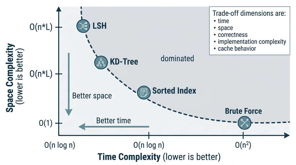
For any problem, the set of viable algorithms forms a Pareto frontier in the complexity trade-off space. An algorithm is Pareto-optimal if no other algorithm is better on every dimension simultaneously. The developer's job is not to find "the best" algorithm (there is no such thing in general) but to identify the Pareto frontier and select the point on it that best matches the application's constraints. Automated benchmarking (Section 15.2) makes this frontier visible; statistical testing tells you which differences are real.
Exercise 15.1.1
You are building a spell-checker that must support two operations on a dictionary of \(n\) words: (1) exact lookup ("is this word valid?") and (2) prefix enumeration ("list all words starting with 'anti'"). A hash map covers operation 1 in \(O(1)\) but cannot help with operation 2. A trie covers both. A sorted array covers both via binary search. Rank these three data structures by filling in a trade-off table with columns for lookup time, prefix query time, insertion time, and memory usage. Which structure is Pareto-optimal for a read-heavy workload with rare insertions?
Hint
For the sorted array, prefix enumeration takes \(O(\log n + r)\) where \(r\) is the number of results, using a binary search to find the first match and then scanning forward. For memory, consider that a trie with shared prefixes can use less space than \(n\) separate strings when prefixes overlap heavily, but more space than a flat sorted array when they do not.
2. The Complexity-Correctness Trade-off Space
A concrete example that runs through the entire chapter makes the trade-off space visible. Suppose you are building a scientific data pipeline that must deduplicate records: given \(n\) records, find all pairs whose similarity exceeds a threshold \(\tau\). This is the all-pairs similarity search problem, which arises in literature deduplication (Chapter 36), chemical compound matching, and entity resolution in knowledge graphs (Chapter 38).
We can enumerate at least four algorithmic strategies, each occupying a different region of the trade-off space:
Strategy 1: Brute force. Compare every pair. Time \(O(n^2 \cdot d)\) where \(d\) is the cost of comparing two records. Space \(O(1)\) beyond the input. Correctness: exact, deterministic. Implementation complexity: minimal (a nested loop). This is the baseline against which all others are measured.
Strategy 2: Sorted index. Sort records by a key, then scan for near-neighbors within a window. Time \(O(n \log n + n \cdot w \cdot d)\) where \(w\) is the expected window size. Space \(O(n)\) for the sorted index. Correctness: exact if the sort key preserves the similarity ordering; approximate otherwise. Implementation: moderate (choosing the right sort key requires domain knowledge).
Strategies 1 and 2 guarantee exact results; the next two trade exactness or worst-case bounds for speed at scale.
Strategy 3: Locality-sensitive hashing (LSH). Hash records into buckets such that similar records collide with high probability. Time \(O(n \cdot L \cdot k)\) for hashing plus \(O(n \cdot b \cdot d)\) for comparing bucket co-members, where \(L\) is the number of hash tables, \(k\) is the hash length, and \(b\) is the average bucket size. Space \(O(n \cdot L)\). Correctness: probabilistic (false negatives with bounded probability). Implementation: complex (tuning \(L\) and \(k\) for desired recall).
Strategy 4: KD-tree / Ball tree. Build a spatial index. Time \(O(n \log n)\) construction, \(O(n \cdot \log n \cdot d)\) query for low \(d\), degrading to \(O(n^2)\) for high \(d\). Space \(O(n)\). Correctness: exact. Implementation: moderate (library-provided, but performance depends heavily on dimensionality).
"""
Four strategies for all-pairs similarity search,
each occupying a different region of the trade-off space.
"""
from dataclasses import dataclass
from enum import Enum

class Correctness(Enum):
    EXACT_DETERMINISTIC = "exact_deterministic"
    EXACT_CONDITIONAL = "exact_conditional"       # exact only if preconditions hold
    PROBABILISTIC = "probabilistic"               # bounded false-negative rate

@dataclass
class AlgorithmProfile:
    """Characterizes one point in the trade-off space."""
    name: str
    time_worst: str       # Big-O as a string for display
    time_average: str
    space: str
    correctness: Correctness
    impl_lines: int       # rough lines-of-code estimate

# Enumerate the candidates for all-pairs similarity search
candidates = [
    AlgorithmProfile(
        name="Brute Force",
        time_worst="O(n^2 * d)",
        time_average="O(n^2 * d)",
        space="O(1)",
        correctness=Correctness.EXACT_DETERMINISTIC,
        impl_lines=8,
    ),
    AlgorithmProfile(
        name="Sorted Index",
        time_worst="O(n^2 * d)",       # worst case: all records in one window
        time_average="O(n log n + n*w*d)",
        space="O(n)",
        correctness=Correctness.EXACT_CONDITIONAL,
        impl_lines=25,
    ),
    AlgorithmProfile(
        name="LSH",
        time_worst="O(n^2 * d)",       # worst case: all hashes collide
        time_average="O(n*L*k + n*b*d)",
        space="O(n * L)",
        correctness=Correctness.PROBABILISTIC,
        impl_lines=60,
    ),
    AlgorithmProfile(
        name="KD-Tree",
        time_worst="O(n^2 * d)",       # high-dimensional degradation
        time_average="O(n log n * d)",
        space="O(n)",
        correctness=Correctness.EXACT_DETERMINISTIC,
        impl_lines=5,                   # library call
    ),
]

# Display the Pareto frontier candidates
for c in candidates:
    print(f"{c.name:15s} | worst: {c.time_worst:15s} | "
          f"avg: {c.time_average:20s} | space: {c.space:8s} | "
          f"{c.correctness.value:20s} | ~{c.impl_lines} lines")
The code above treats algorithm profiles as data rather than prose. This is deliberate: when algorithm selection is a search problem, the candidates should be structured objects that your tools can filter, sort, and visualize. The Discovery Workbench (introduced in Chapter 6) stores these profiles alongside the benchmark results from Section 15.2, creating an auditable record of why a particular algorithm was chosen. The diagram below (Figure 15.1) plots all four candidates on the time-vs-space axes, marking the Pareto frontier that connects the non-dominated strategies.
Step-Through: Pareto Dominance Check
Trace through a dominance check for three algorithm candidates on two axes (time, space). Candidate A: time = 50 ms, space = 200 MB. Candidate B: time = 120 ms, space = 80 MB. Candidate C: time = 90 ms, space = 300 MB.
Compare A vs. B: A is better on time (50 < 120) but worse on space (200 > 80). Neither dominates the other; both survive. Compare A vs. C: A is better on time (50 < 90) and better on space (200 < 300). A dominates C; remove C. Compare B vs. C: B is better on time (120 < 90? No) but better on space (80 < 300). B loses on time, so neither dominates. However, C was already removed by A. Final Pareto frontier: {A, B}. The designer now chooses between A (fast, memory-hungry) and B (slower, memory-frugal) based on the application's constraints.
3. Data Structure Selection
Mapping the Pareto frontier tells you which algorithms survive, but each surviving algorithm assumes a particular way of organizing the underlying data, and that assumption deserves its own analysis.
Every algorithm operates on data structures, and the choice of data structure constrains which algorithms are viable. A hash map enables \(O(1)\) lookup but does not support range queries. A sorted array supports \(O(\log n)\) binary search and efficient range queries but has \(O(n)\) insertion. A skip list (a layered linked list where each layer skips over a geometrically increasing number of elements, enabling binary-search-like performance without tree rotations) offers \(O(\log n)\) expected performance for all operations with simpler concurrency than a balanced tree. The data structure is not merely an implementation detail; it is a design decision that shapes the entire algorithmic strategy.
We can organize data structures into a taxonomy based on the operations they support efficiently. This taxonomy serves as a map for algorithmic exploration: given the operations your problem requires, the taxonomy narrows the set of viable data structures, which in turn narrows the set of viable algorithms.
"""
Data structure taxonomy: maps required operations
to candidate data structures with their complexity profiles.
"""
from typing import Dict, List, Tuple

# Operation -> list of (data_structure, complexity)
OPERATION_MAP: Dict[str, List[Tuple[str, str]]] = {
    "point_lookup": [
        ("hash_map",        "O(1) expected, O(n) worst"),
        ("sorted_array",    "O(log n)"),
        ("balanced_bst",    "O(log n)"),
        ("trie",            "O(k) where k = key length"),
    ],
    "range_query": [
        ("sorted_array",    "O(log n + r) where r = result size"),
        ("balanced_bst",    "O(log n + r)"),
        ("b_tree",          "O(log_B n + r/B) where B = block size"),
        # hash_map intentionally absent: no range support
    ],
    "insert": [
        ("hash_map",        "O(1) amortized (averaged over a sequence of operations)"),
        ("sorted_array",    "O(n)"),
        ("balanced_bst",    "O(log n)"),
        ("skip_list",       "O(log n) expected"),
    ],
    "ordered_iteration": [
        ("sorted_array",    "O(n)"),
        ("balanced_bst",    "O(n) in-order traversal"),
        ("skip_list",       "O(n)"),
        # hash_map: no ordering
    ],
    "prefix_search": [
        ("trie",            "O(k + r) where k = prefix length"),
        ("sorted_array",    "O(log n + r) with binary search"),
    ],
    "nearest_neighbor": [
        ("kd_tree",         "O(log n) for low d, O(n) for high d"),
        ("ball_tree",       "O(log n) adaptive to intrinsic dim (the true number of degrees of freedom in the data, often much less than the ambient dimension)"),
        ("vp_tree",         "O(log n) for metric spaces"),
        ("lsh_index",       "O(1) query, approximate"),
    ],
}

def suggest_structures(required_ops: List[str]) -> Dict[str, int]:
    """Score data structures by how many required operations they support."""
    scores: Dict[str, int] = {}
    for op in required_ops:
        if op not in OPERATION_MAP:
            print(f"Warning: unknown operation '{op}'")
            continue
        for ds, _complexity in OPERATION_MAP[op]:
            scores[ds] = scores.get(ds, 0) + 1
    # Sort by coverage (descending)
    return dict(sorted(scores.items(), key=lambda x: -x[1]))

# Example: a problem requiring lookup, range queries, and insertion
needed = ["point_lookup", "range_query", "insert"]
ranked = suggest_structures(needed)
for ds, coverage in ranked.items():
    print(f"{ds:20s}: covers {coverage}/{len(needed)} operations")
# Output:
# balanced_bst        : covers 3/3 operations
# sorted_array        : covers 3/3 operations
# hash_map            : covers 2/3 operations
# b_tree              : covers 1/3 operations
# skip_list           : covers 1/3 operations
# trie                : covers 1/3 operations
The recommender is deliberately simple; a production version would weight operations by frequency (99% reads vs. 50/50 read-write yields different answers) and account for constant factors. The methodology matters: enumerate required operations, match against data structure capabilities, and narrow the search space before committing to an implementation.
Consider building the citation index for the literature mining pipeline in
Chapter 36.
The index must support: (1) point lookup by Digital Object Identifier (DOI) (\(O(1)\) needed, millions of entries),
(2) range queries by publication year (for filtering), (3) prefix search by author
name (for autocomplete), and (4) ordered iteration by citation count (for ranking).
Running suggest_structures(["point_lookup", "range_query", "prefix_search",
"ordered_iteration"]) surfaces sorted_array and
balanced_bst as top candidates (3/4 coverage each), with trie
contributing the missing prefix search. The practical solution: a composite index
using a hash map for DOI lookup, a B-tree for year ranges (matching the database engine
underneath), and a trie for author prefix search. No single data structure covers all
operations; the discovery process reveals where composites are necessary.
4. Beyond Asymptotic Analysis
Selecting the right data structure narrows the candidate set, but the complexity classes printed next to each candidate can be misleading if taken at face value.
Asymptotic complexity tells you how performance scales as \(n\) grows toward infinity. It says nothing about the constant factors that dominate at practical input sizes, the cache behavior that can make a theoretically slower algorithm faster in practice, or the branch prediction patterns that vary between CPU architectures. An \(O(n \log n)\) merge sort has better worst-case guarantees than \(O(n \log n)\) quicksort, but quicksort is typically faster in practice on most hardware because its sequential access pattern tends to be more cache-friendly, while merge sort's out-of-place merging causes cache misses.
Common Misconception
Misconception: "The algorithm with the better Big-O is always faster." Big-O notation describes the growth rate as \(n\) approaches infinity, not the actual running time at any specific input size. An \(O(n^2)\) algorithm with tiny constant factors will outperform an \(O(n \log n)\) algorithm with large constants for all inputs below the crossover point, which can be in the thousands or even millions depending on implementation details and hardware. Always measure on realistic input sizes before concluding that a lower asymptotic class means faster execution.
The gap between theory and practice has three main sources:
Constant factors. Big-O hides multiplicative constants. An \(O(n)\) algorithm with a constant of 1000 is slower than an \(O(n^2)\) algorithm with a constant of 1 for all \(n < 1000\). The crossover point, where the asymptotically faster algorithm actually becomes faster, is an empirical quantity that must be measured, not assumed.
Cache hierarchy. Modern CPUs have L1 caches (4 cycles), L2 caches (12 cycles), L3 caches (40 cycles), and main memory (200+ cycles). An algorithm that accesses memory sequentially (arrays) can be an order of magnitude faster in practice than one that accesses randomly (linked lists, trees with pointer chasing), even when both have the same asymptotic complexity (the exact factor varies by hardware and access pattern, but 5x to 20x is typical on modern x86 processors). The RAM model assumes uniform memory access cost, which is false on real hardware.
Input distribution. Average-case analysis assumes a distribution over inputs, but the actual distribution in your application may differ. Quicksort's \(O(n^2)\) worst case occurs on already-sorted input, which is common in practice (log files, time-series data, database exports). Randomized algorithms mitigate this by making performance independent of input distribution, at the cost of requiring a random number generator (RNG).
Mental Model
Think of amortized analysis like paying a monthly phone bill versus paying per call. If your plan costs \$60/month for unlimited calls, each individual call is "free," but once a month you pay a lump sum. Some months you make 200 calls (2 cents each, effectively), other months just 10 (6 dollars each, effectively). The per-call cost varies wildly, but the per-call amortized cost over the year is stable and predictable. A dynamic array works the same way: most appends are cheap (just place the element), but occasionally you pay a big "bill" (copy everything to a larger allocation). The amortized cost averages the rare expensive resizes over the many cheap appends, giving a stable \(O(1)\) per operation. The critical subtlety, just as with phone plans, is that the lump-sum payment still happens at a specific moment; if you have a latency deadline on every single call, the average cost is irrelevant.
"""
Demonstrating the crossover point: O(n^2) insertion sort
beats O(n log n) merge sort for small n due to lower constant factors.
"""
import timeit
import statistics

def insertion_sort(arr: list[int]) -> list[int]:
    """O(n^2) but low constant factor, cache-friendly, in-place."""
    result = arr.copy()
    for i in range(1, len(result)):
        key = result[i]
        j = i - 1
        while j >= 0 and result[j] > key:
            result[j + 1] = result[j]
            j -= 1
        result[j + 1] = key
    return result

def merge_sort(arr: list[int]) -> list[int]:
    """O(n log n) guaranteed but higher constant factor, not in-place."""
    if len(arr) <= 1:
        return arr.copy()
    mid = len(arr) // 2
    left = merge_sort(arr[:mid])
    right = merge_sort(arr[mid:])
    return _merge(left, right)

def _merge(left: list[int], right: list[int]) -> list[int]:
    result = []
    i = j = 0
    while i < len(left) and j < len(right):
        if left[i] <= right[j]:
            result.append(left[i])
            i += 1
        else:
            result.append(right[j])
            j += 1
    result.extend(left[i:])
    result.extend(right[j:])
    return result

# Find the crossover point
import random
for n in [5, 10, 20, 50, 100, 200, 500]:
    data = [random.randint(0, 10_000) for _ in range(n)]
    t_ins = statistics.median(
        timeit.repeat(lambda: insertion_sort(data), number=1000, repeat=5)
    )
    t_merge = statistics.median(
        timeit.repeat(lambda: merge_sort(data), number=1000, repeat=5)
    )
    winner = "insertion" if t_ins < t_merge else "merge"
    print(f"n={n:4d} | insertion: {t_ins:.4f}s | merge: {t_merge:.4f}s | winner: {winner}")
sorted() exploits this: Timsort uses insertion sort for small runs.The crossover experiment above is a microcosm of the entire chapter's methodology. We do not argue about which algorithm is "theoretically better." We measure, with enough repetitions to get stable statistics, and let the data speak. Section 15.2 formalizes this approach with proper statistical testing.
The crossover logic above is not merely academic. Python's sorted() and
list.sort() use Timsort, a hybrid algorithm that switches
between merge sort and insertion sort based on run length. Instead of our 50-line
implementation, you call sorted(data) (1 line). Timsort also detects
pre-existing order in the input ("natural runs"), achieving \(O(n)\) on nearly-sorted
data. The library handles the crossover tuning, the run detection, and the galloping
merge optimization internally. Our from-scratch implementations above exist to make
the trade-off space visible; in production, use the library.
5. Systematic Candidate Enumeration
Given a new problem, how do you generate the initial set of algorithm candidates? Textbooks organize algorithms by design paradigm: divide and conquer, dynamic programming, greedy, randomized, approximation. Each paradigm carries assumptions about problem structure that, when satisfied, yield predictable complexity guarantees.
A systematic enumeration asks four questions for each paradigm:

- Does the problem have optimal substructure? If subproblems can be solved independently and their solutions composed, divide-and-conquer or dynamic programming applies. The recurrence relation determines the complexity.
- Does a greedy choice lead to a globally optimal solution? If the matroid structure is present (where a matroid is a combinatorial structure guaranteeing that greedily extending a partial solution always leads to a global optimum, as in minimum spanning trees) or you can prove the greedy-choice property, a greedy algorithm is both correct and efficient. Without this structure, greedy gives an approximation.
- Can randomization break worst-case adversarial inputs? Randomized algorithms trade deterministic guarantees for expected-case performance that is independent of input distribution. Quickselect gives \(O(n)\) expected time for the \(k\)-th element; the deterministic median-of-medians gives \(O(n)\) worst case but with a larger constant.
- Is an approximate answer acceptable? Approximation algorithms trade solution quality for speed. A \((1 + \epsilon)\)-approximation to the traveling salesman problem runs in polynomial time; the exact solution is NP-hard (meaning no known algorithm solves it in polynomial time, and proving or disproving this is one of the central open problems in computer science). Many scientific applications (nearest-neighbor search, clustering) tolerate controlled approximation.
"""
Systematic candidate enumeration: given a problem description,
generate algorithm candidates from design paradigms.
"""
from dataclasses import dataclass, field
from typing import Optional

@dataclass
class ProblemTraits:
    """Properties of the problem that determine which paradigms apply."""
    has_optimal_substructure: bool = False
    has_overlapping_subproblems: bool = False  # if True: DP, not divide-and-conquer
    has_greedy_choice_property: bool = False
    input_adversarial: bool = False            # can adversary choose worst input?
    approximate_ok: bool = False
    epsilon: Optional[float] = None            # approximation tolerance
    max_n: int = 10_000                        # expected input size

@dataclass
class Candidate:
    paradigm: str
    expected_complexity: str
    rationale: str
    risks: list[str] = field(default_factory=list)

def enumerate_candidates(traits: ProblemTraits) -> list[Candidate]:
    """Generate algorithm candidates based on problem traits."""
    candidates = []

    # Brute force is always a candidate (baseline)
    candidates.append(Candidate(
        paradigm="brute_force",
        expected_complexity="varies (often O(n^2) or O(2^n))",
        rationale="Always correct, always simple. Benchmark baseline.",
        risks=["May be too slow for large n"],
    ))

    if traits.has_optimal_substructure and not traits.has_overlapping_subproblems:
        candidates.append(Candidate(
            paradigm="divide_and_conquer",
            expected_complexity="O(n log n) typical",
            rationale="Subproblems are independent; no memoization needed.",
            risks=["Stack depth O(log n)", "Merge step may dominate"],
        ))

    if traits.has_optimal_substructure and traits.has_overlapping_subproblems:
        candidates.append(Candidate(
            paradigm="dynamic_programming",
            expected_complexity="O(n * S) where S = state space size",
            rationale="Subproblems overlap; memoization avoids recomputation.",
            risks=["Space O(S) for the table", "State space may be large"],
        ))

    if traits.has_greedy_choice_property:
        candidates.append(Candidate(
            paradigm="greedy",
            expected_complexity="O(n log n) typical (sort + scan)",
            rationale="Greedy choice is provably safe.",
            risks=["Must verify greedy-choice property holds"],
        ))

    if traits.input_adversarial:
        candidates.append(Candidate(
            paradigm="randomized",
            expected_complexity="expected O(n log n) or better",
            rationale="Randomization breaks adversarial worst cases.",
            risks=["Expected, not guaranteed", "Needs good RNG"],
        ))

    if traits.approximate_ok and traits.epsilon is not None:
        candidates.append(Candidate(
            paradigm="approximation",
            expected_complexity=f"depends on epsilon={traits.epsilon}",
            rationale=f"Trading {traits.epsilon:.0%} quality for polynomial time.",
            risks=["Approximation ratio may not be tight"],
        ))

    return candidates

# Example: all-pairs similarity with approximate tolerance
traits = ProblemTraits(
    has_optimal_substructure=False,
    has_greedy_choice_property=False,
    input_adversarial=True,      # user data can have any distribution
    approximate_ok=True,
    epsilon=0.05,                # 5% false-negative rate acceptable
    max_n=100_000,
)
for c in enumerate_candidates(traits):
    print(f"[{c.paradigm}] {c.expected_complexity}")
    print(f"  Rationale: {c.rationale}")
    print(f"  Risks: {', '.join(c.risks)}\n")
The enumeration function above is a decision support tool, not an oracle. It narrows the search space from "all algorithms ever invented" to a manageable set of paradigm-specific candidates. The next step is to instantiate each paradigm as a concrete implementation, which is where program synthesis (Section 15.2) enters the picture.
Traditionally, algorithm design has been a purely human creative endeavor. Recent work challenges this assumption. AlphaDev (Mankowitz et al., 2023) used deep reinforcement learning to discover sorting algorithms that outperform human-engineered implementations at the assembly instruction level, finding novel swap-and-branch sequences that no human had considered. FunSearch (Romera-Paredes et al., 2024) used LLMs to search the space of programs for mathematical constructions, discovering new solutions to the cap set problem in combinatorics. More recently, AlphaEvolve (DeepMind, 2025) extended this line of work by using an ensemble of large language models to evolve entire codebases, discovering a provably faster algorithm for \(4 \times 4\) complex matrix multiplication (requiring fewer scalar multiplications than any previously known method) and improving the Strassen bound for matrix multiplication that had stood since 1969. AlphaEvolve also found improved constructions for the kissing number problem in geometry and optimized critical scheduling algorithms inside Google's data centers. These results demonstrate that algorithm discovery is a genuine search problem amenable to automated exploration, not merely an exercise in recombining known patterns. The techniques in this chapter, proposing candidates, benchmarking, and selecting winners, are the building blocks of such automated discovery systems. We revisit automated scientific discovery at scale in Chapter 53.
Real-World Application: PostgreSQL Query Planner
PostgreSQL's query planner performs algorithm search on every query execution. Given a SQL query joining three tables, the planner enumerates candidate join strategies (nested loop, hash join, merge join), assigns each a cost estimate based on table statistics (row counts, index availability, value distributions), and selects the plan on the Pareto frontier of estimated I/O cost versus CPU cost. For queries involving many tables, PostgreSQL switches from exhaustive enumeration to its Genetic Query Optimizer (GEQO) because the join-order search space grows factorially. This is the same paradigm-then-data-structure-then-implementation cascade described in this section, running thousands of times per second inside a production database.
6. Amortized Analysis and Hidden Costs
Constant factors and cache effects explain why measured performance diverges from asymptotic predictions on a single operation, but some algorithms spread their costs unevenly across a sequence of operations, introducing a subtler source of surprise.
Some data structures and algorithms have costs that are uneven across operations.
A dynamic array (list in Python) has \(O(1)\) amortized append: most appends
take constant time, but occasionally the array must be resized, costing \(O(n)\). The
amortized cost averages this rare expensive operation over the many cheap ones. For
interactive applications with latency service-level agreements (SLAs), a single \(O(n)\) resize can cause a
visible stutter. For batch processing, the amortized cost is all that matters.
Amortized analysis uses three main techniques, each revealing a different perspective on the cost distribution:
Aggregate analysis computes the total cost of \(n\) operations and divides by \(n\). For a dynamic array starting at size 1 with doubling, the total cost of \(n\) appends is \(n + 1 + 2 + 4 + \ldots + 2^{\lfloor \log n \rfloor} \leq 3n\), giving amortized cost \(O(1)\) per append.
The accounting method assigns each operation a "charge" that may exceed its actual cost. Excess charge is saved as credit on the data structure; expensive operations draw from this credit. Each append is charged 3 units: 1 for the insertion itself, 2 saved as credit. When a resize occurs, the saved credit pays for copying.
The potential method takes a more global view: it defines a potential function \(\Phi\) that assigns a single number to the data structure's current state, much like gravitational potential energy measures how much "stored work" an object has by virtue of its position. The amortized cost of operation \(i\) is \(c_i + \Phi(D_i) - \Phi(D_{i-1})\). For the dynamic array, \(\Phi(D) = 2n - \text{capacity}\) works: it increases by 2 with each append (matching the accounting method's credit) and drops to 0 after a resize.
Checkpoint
So far: amortized analysis has three lenses for the same idea: aggregate analysis divides total cost by operation count, the accounting method pre-charges each operation and banks credit for expensive ones, and the potential method tracks stored work as a single number that rises on cheap operations and drops on expensive ones.
"""
Visualizing amortized costs: actual vs. amortized cost
of dynamic array appends with doubling strategy.
"""
import math

def simulate_dynamic_array(n: int) -> tuple[list[int], list[float]]:
    """
    Simulate n appends to a dynamic array with doubling.
    Returns (actual_costs, running_amortized_costs).
    """
    capacity = 1
    size = 0
    actual_costs = []
    total_cost = 0

    for i in range(n):
        if size == capacity:
            # Resize: copy all elements (cost = capacity) + insert (cost = 1)
            cost = capacity + 1
            capacity *= 2
        else:
            cost = 1
        size += 1
        actual_costs.append(cost)
        total_cost += cost

    running_amortized = [total_cost / (i + 1) for i in range(n)]
    # But the true amortized analysis gives O(1) per operation:
    amortized_bound = [3.0] * n  # the accounting method bound
    return actual_costs, amortized_bound

actual, amortized = simulate_dynamic_array(64)
print("Operation | Actual Cost | Amortized Bound")
print("-" * 45)
for i in [0, 1, 2, 3, 4, 7, 8, 15, 16, 31, 32, 63]:
    print(f"    {i:5d} | {actual[i]:11d} | {amortized[i]:15.1f}")
# Output shows spikes at powers of 2 (resize events)
# while the amortized bound stays constant at 3.0
A widely cited production incident (reported in practitioner forums, though details vary in the retelling) involved a real-time trading system that appended to a
Python list in a hot loop. The system met its 1ms latency target 99.9% of the time,
but every 1024 iterations, a list resize caused a 5ms spike that triggered the
circuit breaker. The fix: pre-allocate the list with [None] * max_size.
Amortized \(O(1)\) is not the same as worst-case \(O(1)\), and your SLA does not care
about averages.
7. Building the Algorithm Search Tree
We can organize the entire algorithm selection process as a search tree. The root is the problem specification. Each level corresponds to a design decision: paradigm selection, data structure choice, implementation variant, and optimization level. Leaves are concrete implementations ready for benchmarking.
"""
Algorithm search tree: organize the selection process
as a tree of decisions leading to concrete implementations.
"""
from dataclasses import dataclass, field
from typing import Optional

@dataclass
class SearchNode:
    """A node in the algorithm search tree."""
    decision: str           # what this level decides
    choice: str             # the specific choice at this node
    rationale: str          # why this choice
    children: list["SearchNode"] = field(default_factory=list)
    is_leaf: bool = False   # leaf nodes are benchmarkable implementations
    impl_ref: Optional[str] = None  # reference to implementation function

    def display(self, indent: int = 0) -> None:
        prefix = "  " * indent
        marker = "[IMPL]" if self.is_leaf else ""
        print(f"{prefix}{self.decision}: {self.choice} {marker}")
        if self.rationale:
            print(f"{prefix}  reason: {self.rationale}")
        for child in self.children:
            child.display(indent + 1)

# Build the search tree for all-pairs similarity
root = SearchNode(
    decision="Problem",
    choice="All-pairs similarity (n=100k, d=128, tau=0.8)",
    rationale="Record deduplication in literature pipeline",
    children=[
        SearchNode(
            decision="Paradigm",
            choice="Brute force",
            rationale="Baseline, always correct",
            children=[
                SearchNode(
                    decision="Implementation",
                    choice="NumPy vectorized cosine",
                    rationale="Exploit BLAS (Basic Linear Algebra Subprograms) for matrix multiply",
                    is_leaf=True,
                    impl_ref="brute_force_numpy",
                ),
            ],
        ),
        SearchNode(
            decision="Paradigm",
            choice="Spatial indexing",
            rationale="Exploit metric structure of similarity",
            children=[
                SearchNode(
                    decision="Data structure",
                    choice="Ball tree",
                    rationale="Adapts to intrinsic dimensionality",
                    children=[
                        SearchNode(
                            decision="Implementation",
                            choice="scikit-learn BallTree",
                            rationale="Mature, optimized C implementation",
                            is_leaf=True,
                            impl_ref="balltree_sklearn",
                        ),
                    ],
                ),
            ],
        ),
        SearchNode(
            decision="Paradigm",
            choice="Hashing (approximate)",
            rationale="Trade recall for speed at large n",
            children=[
                SearchNode(
                    decision="Data structure",
                    choice="LSH with random projections",
                    rationale="Well-suited for cosine similarity",
                    children=[
                        SearchNode(
                            decision="Implementation",
                            choice="datasketch MinHashLSH",
                            rationale="Production-grade, tunable recall",
                            is_leaf=True,
                            impl_ref="lsh_datasketch",
                        ),
                    ],
                ),
            ],
        ),
    ],
)

root.display()
The search tree makes the decision space explicit and auditable. When a benchmark reveals that the chosen algorithm is too slow, you do not start from scratch. You walk back up the tree to the relevant decision node and explore an alternative branch. This structured backtracking is far more efficient than ad-hoc algorithm swapping, and it integrates naturally with the architectural decision records from Chapter 14.
Algorithm selection is not a single choice. It is a cascade of decisions: paradigm, data structure, implementation variant, optimization level. Each level constrains the next. Modeling this cascade as a search tree (1) makes the decision space visible, (2) enables systematic exploration of alternatives when the first choice does not meet performance targets, and (3) creates a traceable record linking performance measurements to the design decisions that produced them. The Discovery Workbench stores the search tree alongside benchmark results, forming the algorithmic counterpart to the architecture decision records in Chapter 14.
Try It: Build and Benchmark Your Own Trade-off Frontier
Put the concepts from this section into practice by constructing a Pareto frontier for a concrete search problem using only Python's standard library and NumPy.
- Define the problem. Generate a dataset of 10,000 random 16-dimensional
vectors using
numpy.random.default_rng(42).standard_normal((10_000, 16)). Your task: for each vector, find its 5 nearest neighbors by Euclidean distance. - Implement three candidates. Write (a) a brute-force solution using
numpy.linalg.normwith broadcasting, (b) a sorted-projection solution that sorts on the first coordinate and searches within a window, and (c) ascipy.spatial.KDTreesolution (one library call). - Measure the trade-off axes. For each candidate, record wall-clock time
(use
timeitwith at least 3 repetitions), peak memory (usetracemalloc), and recall at \(k{=}5\) (fraction of true neighbors found, using brute force as ground truth). - Plot the frontier. Create a scatter plot with time on the x-axis and memory on the y-axis, labeling each point with the algorithm name and its recall. Identify which candidates are Pareto-optimal and which are dominated.
- Vary the dimensionality. Repeat steps 1 through 4 with \(d = 64\) and \(d = 256\). Observe how the KD-tree's position on the frontier shifts as dimensionality increases (the "curse of dimensionality," where the volume of the space grows so fast with each added dimension that data points become nearly equidistant, rendering spatial partitioning ineffective).
Lab: Crossover Point Hunter
Goal: Empirically find the input size \(n^*\) at which an \(O(n \log n)\) algorithm overtakes an \(O(n^2)\) algorithm, and observe how hardware and data characteristics shift that crossover.
Tools: Python 3.10+, NumPy, and timeit (all in the standard
scientific stack; no GPU required).
Procedure (20 minutes): Implement insertion sort and merge sort from this section. Benchmark both on random integer arrays for $n \in \{8, 16, 32, 64, 128, 256, 512, 1024\}$, recording median wall-clock time over 50 repetitions per size. Plot time versus \(n\) on a log-log scale and identify the crossover \(n^*\).
What to vary: (1) Change the input distribution from uniform random to
90% pre-sorted (sort the array, then shuffle 10% of positions at random). (2) Switch
from Python lists to NumPy arrays. (3) If time permits, add Python's built-in
sorted() as a third curve.
What to observe: How does pre-sorted input shift \(n^*\)? Does the NumPy
array representation change constant factors enough to move the crossover? Where does
Timsort (sorted()) sit relative to your two hand-rolled implementations,
and does it ever lose to either one?
Exercises
- Conceptual: For the problem of finding the top-\(k\) elements in an unsorted array, enumerate at least four algorithm candidates from different design paradigms. Characterize each by its time complexity, space complexity, and correctness guarantee. At what value of \(k\) relative to \(n\) does the Pareto frontier shift from favoring partial-sort approaches to favoring full-sort approaches? Connect your analysis to the discovery-as-search framework from Chapter 1.
-
Coding: Extend the
suggest_structuresfunction to accept operation frequencies (e.g., "90% lookups, 5% inserts, 5% range queries") and weight data structure scores accordingly. Test it with three different workload profiles and verify that the recommendations change sensibly. Add amemory_budgetparameter that filters out data structures known to exceed a given space bound. - Analysis: Run the crossover-point experiment (insertion sort vs. merge sort) on your machine. Record the crossover \(n\) value. Then repeat with data that is 90% pre-sorted (simulate by sorting, then randomly perturbing 10% of elements). How does pre-existing order change the crossover point? Explain the result in terms of insertion sort's \(O(n)\) best case on sorted input and Timsort's run-detection optimization.
What's Next
With the trade-off space mapped and candidates enumerated, Section 15.2: Program Synthesis and Benchmarking tackles two questions: how do you generate correct implementations of each candidate (program synthesis with property-based testing), and how do you measure their performance with enough rigor to make defensible claims (benchmarking methodology with statistical hypothesis testing)?