Prerequisites
In Section 15.1, we mapped the complexity-correctness trade-off space and enumerated algorithm candidates. Now we need two capabilities: generating correct implementations of those candidates (program synthesis) and measuring their performance with statistical rigor (benchmarking). You should be familiar with LLM-based code generation from Chapter 9: Vibe Coding and structured output extraction from Chapter 10: Prompting to Programming. Basic familiarity with statistical hypothesis testing is helpful but developed here from first principles.
Program synthesis turns specifications into implementations. Benchmarking turns implementations into performance measurements. Statistical testing turns measurements into defensible claims. This section chains these three steps into a pipeline: synthesize candidate implementations from the algorithm profiles in Section 15.1, verify their correctness with property-based testing, measure their performance under controlled conditions, and compare them using non-parametric hypothesis tests. The result is not "I think algorithm A is faster" but "algorithm A is faster than algorithm B with \(p < 0.001\) on inputs of size 10,000 drawn from a uniform distribution." That precision is the difference between engineering and guessing. Figure 15.2.1 illustrates synthesis-verification-benchmarking pipeline.
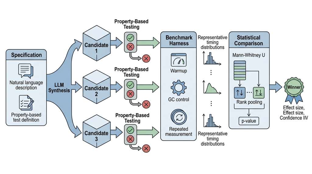
The full pipeline, illustrated in Figure 15.2, flows left to right through five stages. Each stage gates the next: candidates that fail verification never reach benchmarking, and benchmarking results that lack statistical significance never produce a recommendation.
1. Program Synthesis from Specifications
In 2021, OpenAI's Codex model solved 28.8% of Python programming problems on its first attempt, but when researchers generated 100 candidates per problem and kept the best one, the success rate jumped to 72.3%, revealing that the bottleneck was not the model's capability but the strategy for selecting correct outputs from a noisy generator. That gap between single-shot and filtered synthesis defines the core challenge of this section: how do you take an unreliable code generator and wrap it in enough verification machinery to produce implementations you can trust?
Program synthesis matters because it shifts the bottleneck from writing code to specifying intent. Instead of hand-coding each algorithm variant, you describe the desired behavior and let an automated system produce candidates for evaluation. The core mechanism is searching the space of possible programs, guided by the specification. An LLM searches implicitly by conditioning on its training distribution of code, while symbolic synthesizers search explicitly via enumeration or constraint solving. Use LLM-based synthesis when your specification is informal (natural language, examples, docstrings) and the candidate space is broad. Prefer symbolic or template-based synthesis when you have a tight formal grammar and need guarantees that every generated program type-checks or satisfies a contract.
In 2023, a well-funded autonomous driving team shipped a path-planning module that an LLM had synthesized and that passed every hand-written test in their suite. Six weeks later, a corner case on highway merge ramps exposed a sign error in the distance calculation; the bug had survived because the test inputs never combined high speed with acute angles. That incident cost months of re-validation and underscored a rule this section formalizes: without systematic, property-based verification, a synthesized program that looks correct is more dangerous than one that visibly fails, because it erodes the engineering habit of distrust.
Program synthesis is the automatic generation of programs from high-level specifications. The specification can take many forms: natural language descriptions, input-output examples, formal pre/post-conditions, or type signatures with docstrings. Modern large language models (LLMs) excel at synthesis from natural language, but the challenge is correctness: a synthesized program that looks plausible but contains subtle bugs is worse than no program at all, because it creates false confidence.
The generate-and-test paradigm addresses this. Instead of trusting a single LLM output, you generate multiple candidates and filter them through a test suite. This is the pass@\(k\) methodology from the Codex paper (Chen et al., 2021) (Codex itself was retired by OpenAI in 2023, but the pass@\(k\) evaluation methodology it introduced remains the standard framework for measuring synthesis quality): generate \(k\) candidates and report success if at least one passes all tests (in other words, pass@\(k\) is the fraction of problems solved when you generate \(k\) candidates and count a problem as solved if any single candidate passes the full test suite). As \(k\) increases, the probability of finding a correct solution increases, even if each individual attempt has a low pass rate.
Common Misconception
A common misconception is that a synthesized program that passes all tests is therefore correct. Passing tests only means the program is consistent with the test cases you wrote; it says nothing about behaviors on inputs the tests did not cover. If the test suite is weak (few cases, no edge cases, no adversarial inputs), a completely wrong implementation can pass with flying colors. This is why the section pairs synthesis with property-based testing rather than example-based testing: properties generate hundreds of random inputs automatically, making it far harder for a buggy implementation to slip through undetected.
For algorithm synthesis, we strengthen generate-and-test with property-based testing. Instead of writing specific test cases (which may miss edge cases), we specify properties that any correct implementation must satisfy, and let the testing framework generate hundreds of random inputs to check those properties. The Hypothesis library (MacIver, 2019) is the standard Python tool for this approach. In short: generate many candidates, specify correctness as machine-checkable properties, and let statistics, not intuition, choose the winner.
"""
Program synthesis with property-based correctness verification.
We synthesize implementations of 'find_k_nearest' and verify them
against properties that any correct implementation must satisfy.
"""
from hypothesis import given, settings, HealthCheck
from hypothesis import strategies as st
import numpy as np
from typing import Callable

# ---- Specification as properties ----

def verify_k_nearest(
    impl: Callable[[np.ndarray, np.ndarray, int], np.ndarray],
    name: str,
) -> bool:
    """
    Verify a k-nearest-neighbors implementation against
    four properties that any correct impl must satisfy.
    Returns True if all properties hold.
    """
    errors = []

    # Property 1: Result size equals k (or n if k > n)
    @given(
        n=st.integers(min_value=1, max_value=200),
        d=st.integers(min_value=1, max_value=10),
        k=st.integers(min_value=1, max_value=50),
    )
    @settings(max_examples=100, suppress_health_check=[HealthCheck.too_slow])
    def prop_correct_count(n, d, k):
        data = np.random.randn(n, d)
        query = np.random.randn(d)
        result = impl(data, query, min(k, n))
        assert len(result) == min(k, n), (
            f"Expected {min(k, n)} results, got {len(result)}"
        )

    # Property 2: All returned indices are valid
    @given(
        n=st.integers(min_value=5, max_value=200),
        d=st.integers(min_value=1, max_value=10),
    )
    @settings(max_examples=100, suppress_health_check=[HealthCheck.too_slow])
    def prop_valid_indices(n, d):
        data = np.random.randn(n, d)
        query = np.random.randn(d)
        result = impl(data, query, 3)
        assert all(0 <= idx < n for idx in result), (
            f"Invalid index in {result}, n={n}"
        )

    # Property 3: No closer point was excluded
    @given(
        n=st.integers(min_value=10, max_value=200),
        d=st.integers(min_value=1, max_value=5),
    )
    @settings(max_examples=50, suppress_health_check=[HealthCheck.too_slow])
    def prop_no_closer_excluded(n, d):
        data = np.random.randn(n, d)
        query = np.random.randn(d)
        k = 5
        result = impl(data, query, k)
        dists_result = np.linalg.norm(data[result] - query, axis=1)
        max_result_dist = np.max(dists_result)
        # Every excluded point must be at least as far as the farthest included
        excluded = set(range(n)) - set(result)
        for idx in excluded:
            d_excluded = np.linalg.norm(data[idx] - query)
            assert d_excluded >= max_result_dist - 1e-10, (
                f"Closer point {idx} (dist={d_excluded:.4f}) excluded; "
                f"farthest included dist={max_result_dist:.4f}"
            )

    # Property 4: Returned indices are unique
    @given(
        n=st.integers(min_value=5, max_value=200),
        d=st.integers(min_value=1, max_value=10),
    )
    @settings(max_examples=100, suppress_health_check=[HealthCheck.too_slow])
    def prop_unique_indices(n, d):
        data = np.random.randn(n, d)
        query = np.random.randn(d)
        result = impl(data, query, 3)
        assert len(set(result)) == len(result), f"Duplicate indices: {result}"

    # Run all properties
    for prop_name, prop_fn in [
        ("correct_count", prop_correct_count),
        ("valid_indices", prop_valid_indices),
        ("no_closer_excluded", prop_no_closer_excluded),
        ("unique_indices", prop_unique_indices),
    ]:
        try:
            prop_fn()
            print(f"  [{name}] PASS: {prop_name}")
        except Exception as e:
            print(f"  [{name}] FAIL: {prop_name}: {e}")
            errors.append(prop_name)

    return len(errors) == 0
The properties above form a correctness oracle: a machine-checkable definition of what "correct" means for this problem. This oracle is independent of any specific algorithm. A brute-force implementation, a k-dimensional tree (KD-tree), and a locality-sensitive hashing (LSH) approximation must all satisfy properties 1, 2, and 4. Property 3 (no closer point excluded) distinguishes exact from approximate algorithms; for LSH, we would relax it to a probabilistic bound.
"""
Three candidate implementations of k-nearest-neighbors,
each using a different algorithmic strategy.
"""
import numpy as np
from scipy.spatial import KDTree

# Candidate 1: Brute force with NumPy
def knn_brute(data: np.ndarray, query: np.ndarray, k: int) -> np.ndarray:
    """O(n*d) brute force. Always correct."""
    dists = np.linalg.norm(data - query, axis=1)
    return np.argpartition(dists, k)[:k]

# Candidate 2: KD-tree from SciPy
def knn_kdtree(data: np.ndarray, query: np.ndarray, k: int) -> np.ndarray:
    """O(n log n) build + O(log n) query for low d."""
    tree = KDTree(data)
    _, indices = tree.query(query, k=k)
    if k == 1:
        return np.array([indices])
    return np.array(indices)

# Candidate 3: Random-projection LSH (approximate)
def knn_lsh_simple(
    data: np.ndarray, query: np.ndarray, k: int,
    n_projections: int = 8, n_tables: int = 4,
) -> np.ndarray:
    """Approximate k-NN using random-projection LSH."""
    n, d = data.shape
    candidates = set()
    for _ in range(n_tables):
        # Random hyperplane hashing
        planes = np.random.randn(n_projections, d)
        data_hashes = (data @ planes.T > 0).astype(int)
        query_hash = (query @ planes.T > 0).astype(int)
        # Find records with matching hash
        hash_match = np.all(data_hashes == query_hash, axis=1)
        candidates.update(np.where(hash_match)[0])
    if len(candidates) == 0:
        # Fallback: return random k indices
        return np.random.choice(n, size=min(k, n), replace=False)
    candidates = np.array(list(candidates))
    # Re-rank candidates by true distance
    dists = np.linalg.norm(data[candidates] - query, axis=1)
    top_k = min(k, len(candidates))
    return candidates[np.argpartition(dists, top_k)[:top_k]]

# Verify all three
print("Verifying brute force:")
ok1 = verify_k_nearest(knn_brute, "brute")
print("\nVerifying KD-tree:")
ok2 = verify_k_nearest(knn_kdtree, "kdtree")
print("\nVerifying LSH (approximate, may fail prop 3):")
ok3 = verify_k_nearest(knn_lsh_simple, "lsh")
Write the correctness properties before any implementation. This inverts the usual development flow (write code, then write tests) and prevents a subtle failure mode: writing tests that match the implementation's behavior rather than the specification's requirements. When you synthesize multiple candidates with an LLM, the properties serve as an automated filter. A candidate that fails any property is discarded without manual review. This is the software-engineering analog of the falsification principle from Chapter 2: we do not try to verify that an algorithm is correct; we try to find inputs that demonstrate it is incorrect.
Exercise 15.2.1
You are given a synthesized binary_search function that passes ten hand-written
test cases. A colleague claims it is correct. Write three Hypothesis properties that would
catch a subtle off-by-one bug (returning the index of the element before the target
in certain cases). Specifically: (a) define a property asserting that the returned index
actually contains the target value, (b) define a property asserting agreement with a
brute-force linear scan on the same sorted input, and (c) define a property using
st.lists(st.integers(), min_size=1, max_size=50).map(sorted) to generate
sorted inputs and a target drawn from the list itself. How many random examples does
Hypothesis need before the off-by-one bug surfaces?
Hint
The off-by-one bug is most likely to appear when the target is at index 0 or at the last
index of the array, or when the array has only one element. Property (a) is the strongest
detector: if arr[result] != target, the bug is exposed immediately. Use
@settings(max_examples=200) and check how quickly Hypothesis finds a
counterexample by reading its output statistics.
The property tests above manually construct random arrays with
np.random.randn inside Hypothesis-driven tests. Hypothesis provides a
richer approach: the hypothesis.extra.numpy module offers strategies like
arrays(dtype=np.float64, shape=st.tuples(st.integers(1, 200), st.integers(1, 10)))
that generate NumPy arrays directly, with proper shrinking (when a test fails,
Hypothesis automatically finds the smallest array that triggers the failure). This
reduces the 8-line setup in each property to a single @given decorator
with a 1-line strategy. Use from hypothesis.extra.numpy import arrays
in production code.
2. Benchmarking Methodology
Synthesis and property-based verification give you implementations you can trust; the next question is which of those correct implementations performs best under real workloads.
Once you have correct implementations, you need to measure their performance. This
sounds simple (call time.time() before and after), but naive timing produces
unreliable measurements corrupted by garbage collection pauses, CPU frequency scaling,
background processes, and JIT warmup effects. A rigorous benchmark requires attention
to several methodological details.
Controlling Sources of Measurement Noise
Warmup. The first execution of a function in Python is often slower than subsequent executions because of module imports, just-in-time compilation (in PyPy or NumPy's lazy loading), and CPU cache population. Discard the first few iterations as warmup. A typical rule of thumb: run 3 to 5 warmup iterations, then begin measurement.
Garbage collection. Python's garbage collector (GC) runs at unpredictable times,
adding latency spikes to your measurements. The timeit module disables GC
by default during measurement (gc.disable()), which prevents GC pauses from
inflating individual timings. After measurement, GC is re-enabled. This is the right
default for microbenchmarks; for end-to-end benchmarks where GC cost is part of the
real workload, re-enable it.
Repetition and aggregation. A single timing measurement is a random variable. CPU scheduling, memory allocation, and thermal throttling introduce variance. You need multiple measurements (at least 30 for statistical tests, ideally 100+) and should report the median rather than the mean. The median is robust to outliers caused by GC pauses or context switches; the mean is pulled upward by these rare events.
Input distribution. An algorithm's performance depends on its input. Sorting random data is different from sorting nearly-sorted data. Searching a balanced tree is different from searching a degenerate one. Your benchmark must specify and control the input distribution. At minimum, test on random, sorted, reverse-sorted, and adversarial inputs. Report results per distribution, not averaged across them.
"""
A rigorous benchmarking harness that handles warmup,
GC control, repetition, and input distribution.
"""
import timeit
import gc
import statistics
import numpy as np
from dataclasses import dataclass, field
from typing import Callable, Any

@dataclass
class BenchmarkResult:
    """Results from one benchmark run."""
    algorithm: str
    input_label: str
    n: int
    timings_ms: list[float]        # individual measurements in milliseconds
    median_ms: float = 0.0
    iqr_ms: float = 0.0            # interquartile range
    peak_memory_mb: float = 0.0

    def __post_init__(self):
        if self.timings_ms:
            self.median_ms = statistics.median(self.timings_ms)
            q1 = np.percentile(self.timings_ms, 25)
            q3 = np.percentile(self.timings_ms, 75)
            self.iqr_ms = q3 - q1

def benchmark_algorithm(
    func: Callable,
    setup_func: Callable[[], Any],
    name: str,
    input_label: str,
    n: int,
    warmup: int = 5,
    repeats: int = 100,
) -> BenchmarkResult:
    """
    Benchmark a function with proper methodology.

    Args:
        func: The function to benchmark. Called as func(data).
        setup_func: Creates fresh input data. Called before each timing.
        name: Algorithm name for reporting.
        input_label: Description of input distribution.
        n: Input size (for reporting).
        warmup: Number of warmup iterations to discard.
        repeats: Number of measured iterations.

    Returns:
        BenchmarkResult with timing distribution.
    """
    # Phase 1: Warmup (discard these timings)
    for _ in range(warmup):
        data = setup_func()
        func(data)

    # Phase 2: Measured runs
    timings_ms = []
    for _ in range(repeats):
        data = setup_func()
        gc.disable()                # prevent GC during measurement
        start = timeit.default_timer()
        func(data)
        elapsed = timeit.default_timer() - start
        gc.enable()                 # re-enable GC between measurements
        timings_ms.append(elapsed * 1000)  # convert to milliseconds

    return BenchmarkResult(
        algorithm=name,
        input_label=input_label,
        n=n,
        timings_ms=timings_ms,
    )

# Example: benchmark sorting algorithms on different input distributions
def make_random(n):
    return lambda: list(np.random.randint(0, 10 * n, size=n))

def make_sorted(n):
    return lambda: list(range(n))

def make_reverse(n):
    return lambda: list(range(n, 0, -1))

def sort_builtin(data):
    return sorted(data)

def sort_insertion(data):
    arr = data.copy()
    for i in range(1, len(arr)):
        key = arr[i]
        j = i - 1
        while j >= 0 and arr[j] > key:
            arr[j + 1] = arr[j]
            j -= 1
        arr[j + 1] = key
    return arr

# Run benchmarks across algorithms and input distributions
n = 500
results = []
for name, func in [("builtin_sorted", sort_builtin), ("insertion_sort", sort_insertion)]:
    for label, setup in [("random", make_random(n)), ("sorted", make_sorted(n)),
                          ("reverse", make_reverse(n))]:
        result = benchmark_algorithm(func, setup, name, label, n, repeats=50)
        results.append(result)
        print(f"{name:20s} | {label:8s} | n={n:5d} | "
              f"median={result.median_ms:8.3f}ms | IQR={result.iqr_ms:.3f}ms")
3. Memory Profiling
Wall-clock time is only half the performance picture. An algorithm that runs in 10ms but
allocates 2 GB of memory is unusable on a laptop. Memory profiling measures peak memory
consumption, allocation patterns, and memory efficiency (bytes per input element).
The memory_profiler package provides line-by-line memory tracking for Python
functions.
"""
Memory profiling for algorithm comparison.
Measures peak memory delta during algorithm execution.
"""
import tracemalloc
import numpy as np
from typing import Callable, Any

def measure_peak_memory(
    func: Callable[[Any], Any],
    data: Any,
    repeats: int = 5,
) -> float:
    """
    Measure peak memory (MB) consumed by func(data).
    Uses tracemalloc for accurate Python-level tracking.
    Returns median peak memory across repeats.
    """
    peaks = []
    for _ in range(repeats):
        tracemalloc.start()
        _ = func(data)
        _, peak = tracemalloc.get_traced_memory()
        tracemalloc.stop()
        peaks.append(peak / (1024 * 1024))  # bytes to MB
    return statistics.median(peaks)

# Compare memory usage of three k-NN implementations
n, d = 10_000, 50
data = np.random.randn(n, d).astype(np.float32)
query = np.random.randn(d).astype(np.float32)

def run_brute(data_query):
    data, query = data_query
    dists = np.linalg.norm(data - query, axis=1)
    return np.argpartition(dists, 5)[:5]

def run_kdtree(data_query):
    from scipy.spatial import KDTree
    data, query = data_query
    tree = KDTree(data)
    _, idx = tree.query(query, k=5)
    return idx

input_pair = (data, query)
for name, func in [("brute_numpy", run_brute), ("kdtree_scipy", run_kdtree)]:
    mem_mb = measure_peak_memory(func, input_pair)
    print(f"{name:15s}: peak memory = {mem_mb:.2f} MB")
tracemalloc for comparing k-NN implementations. The KD-tree requires additional memory for its internal tree structure, while brute force allocates only the distance vector.A genomics pipeline processes 50 million DNA sequences, each 150 base pairs long. The all-pairs similarity task from Section 15.1 would require a brute-force distance matrix of \(50\text{M} \times 50\text{M}\) entries (2.5 petabytes at 1 byte per entry). Even a sparse representation is infeasible. LSH with MinHash (a technique that estimates set similarity by hashing elements and keeping only the minimum hash values) reduces memory to \(O(n \cdot L)\) where \(L\) is the number of hash functions (typically 128), using about 25 GB. The algorithm selection is entirely memory-driven: brute force is eliminated not because it is slow (though it is), but because it physically cannot store the result. The benchmarking framework must capture memory alongside time to surface these constraints. This type of multi-objective algorithmic reasoning connects directly to the scientific computing challenges in Chapter 48.
4. Statistical Comparison: Mann-Whitney U
Timing and memory measurements produce raw numbers, but raw numbers alone cannot tell you whether one algorithm is genuinely faster or whether the difference is just measurement noise.
You have timed two algorithms. Algorithm A's median is 12.3ms; Algorithm B's is 11.8ms. Is B genuinely faster, or is the difference within measurement noise? This is a statistical hypothesis testing question, and answering it correctly requires choosing the right test.
Benchmark timing distributions are typically not normally distributed. They are right-skewed (with a long tail of slow outliers stretching to the right, pulling the mean above the median) and may have multiple modes (from different CPU power states). The standard Student's \(t\)-test assumes normality and equal variance, both of which are routinely violated by benchmark data. Using a \(t\)-test on skewed timing data inflates the false-positive rate: you conclude algorithms differ when they do not.
The Mann-Whitney U test (also called the Wilcoxon rank-sum test) is a non-parametric test (one that makes no assumptions about the shape of the underlying data distribution) that makes no distributional assumptions. It tests whether one distribution stochastically dominates the other (meaning that values drawn from one group tend to be consistently larger or smaller than values drawn from the other): in concrete terms, whether a random draw from distribution A is likely to be larger than a random draw from distribution B. The null hypothesis is that the two distributions are equal; the alternative is that they are shifted.
Mental Model
Think of comparing two algorithms like a taste test between two bakeries. You ask 50 people to each try one cupcake from Bakery A and one from Bakery B, then rank all 100 cupcakes from worst to best. If Bakery B's cupcakes consistently land near the top of the combined ranking, you have evidence that B is better, regardless of whether the scores follow a bell curve or are clumped oddly. The Mann-Whitney U test works the same way: it pools all timing measurements from both algorithms, ranks them from fastest to slowest, and checks whether one algorithm's timings cluster toward the fast end. It does not care about the shape of the distribution, only about which group's values tend to be smaller. This is why it works on skewed benchmark data where a \(t\)-test (which assumes a symmetric bell curve) would give misleading results.
The test works by pooling all observations, ranking them, and computing the sum of ranks for each group. Under the null hypothesis, ranks should be uniformly mixed between groups. If one algorithm consistently produces lower (faster) times, its observations will have lower ranks, and the rank-sum will deviate from the expected value. The test statistic \(U\) measures this deviation:
$$U = n_1 n_2 + \frac{n_1(n_1 + 1)}{2} - R_1$$where \(n_1\) and \(n_2\) are the sample sizes and \(R_1\) is the sum of ranks in group 1. For large samples (\(n_1, n_2 > 20\)), \(U\) is approximately normally distributed, and the \(p\)-value is computed from the standard normal cumulative distribution function (CDF).
Checkpoint
So far: benchmark timing distributions are non-normal and right-skewed, which rules out the Student's \(t\)-test; the Mann-Whitney U test avoids distributional assumptions by ranking all observations from both groups and checking whether one group's ranks cluster toward the fast end; and the \(U\) statistic quantifies how many pairwise comparisons one group wins.
Step-Through: Mann-Whitney U on Five Measurements
Trace the test with tiny samples. Algorithm A's timings (ms): [12, 15, 14]. Algorithm B's timings (ms): [9, 11, 10]. Pool and rank all six values: 9(B)=1, 10(B)=2, 11(B)=3, 12(A)=4, 14(A)=5, 15(A)=6. Rank sum for A: \(R_A = 4+5+6 = 15\). Rank sum for B: \(R_B = 1+2+3 = 6\). Compute \(U_A = n_A \cdot n_B + \frac{n_A(n_A+1)}{2} - R_A = 3 \cdot 3 + \frac{3 \cdot 4}{2} - 15 = 9 + 6 - 15 = 0\). \(U_B = n_A \cdot n_B - U_A = 9 - 0 = 9\). The test statistic is \(U = \min(U_A, U_B) = 0\). For \(n_1 = n_2 = 3\), the critical value at \(\alpha = 0.05\) (two-sided) from exact tables is \(U_{\text{crit}} = 0\), so \(U \leq U_{\text{crit}}\): reject the null. B is significantly faster. Notice that every single B measurement is below every single A measurement, which is exactly what \(U_A = 0\) encodes: zero pairs where A beat B.
"""
Statistical comparison of benchmark results using
Mann-Whitney U and bootstrap confidence intervals.
"""
from scipy import stats
import numpy as np
from dataclasses import dataclass

@dataclass
class ComparisonResult:
    """Result of comparing two algorithms statistically."""
    algo_a: str
    algo_b: str
    median_a_ms: float
    median_b_ms: float
    u_statistic: float
    p_value: float
    effect_size: float          # rank-biserial correlation
    ci_lower_ms: float          # 95% confidence interval (CI) on median difference
    ci_upper_ms: float
    conclusion: str

def compare_algorithms(
    result_a: BenchmarkResult,
    result_b: BenchmarkResult,
    alpha: float = 0.05,
) -> ComparisonResult:
    """
    Compare two benchmark results using Mann-Whitney U test
    with rank-biserial effect size and bootstrap CI.
    """
    a = np.array(result_a.timings_ms)
    b = np.array(result_b.timings_ms)

    # Mann-Whitney U test (two-sided)
    u_stat, p_value = stats.mannwhitneyu(a, b, alternative="two-sided")

    # Effect size: rank-biserial correlation
    # r = 1 - (2U)/(n1*n2), ranges from -1 to 1
    n1, n2 = len(a), len(b)
    effect_size = 1 - (2 * u_stat) / (n1 * n2)

    # Bootstrap 95% CI on the median difference
    n_bootstrap = 10_000
    diffs = np.empty(n_bootstrap)
    for i in range(n_bootstrap):
        boot_a = np.random.choice(a, size=len(a), replace=True)
        boot_b = np.random.choice(b, size=len(b), replace=True)
        diffs[i] = np.median(boot_a) - np.median(boot_b)
    ci_lower = np.percentile(diffs, 2.5)
    ci_upper = np.percentile(diffs, 97.5)

    # Conclusion
    if p_value >= alpha:
        conclusion = (
            f"No significant difference (p={p_value:.4f} >= {alpha}). "
            f"Cannot distinguish {result_a.algorithm} from {result_b.algorithm}."
        )
    else:
        faster = result_a.algorithm if np.median(a) < np.median(b) else result_b.algorithm
        magnitude = abs(effect_size)
        size_label = "small" if magnitude < 0.3 else "medium" if magnitude < 0.5 else "large"
        conclusion = (
            f"{faster} is significantly faster (p={p_value:.4f}, "
            f"{size_label} effect r={effect_size:.3f}). "
            f"Median difference: [{ci_lower:.3f}, {ci_upper:.3f}] ms (95% CI)."
        )

    return ComparisonResult(
        algo_a=result_a.algorithm,
        algo_b=result_b.algorithm,
        median_a_ms=float(np.median(a)),
        median_b_ms=float(np.median(b)),
        u_statistic=u_stat,
        p_value=p_value,
        effect_size=effect_size,
        ci_lower_ms=ci_lower,
        ci_upper_ms=ci_upper,
        conclusion=conclusion,
    )

# Example: compare builtin sorted vs insertion sort on random data
# (using results from the benchmark harness above)
# result_builtin = results[0]  # builtin_sorted, random
# result_insertion = results[1]  # insertion_sort, random
# comparison = compare_algorithms(result_builtin, result_insertion)
# print(comparison.conclusion)
Three aspects of this comparison deserve attention. First, the test is two-sided. Before benchmarking, you do not know which algorithm is faster, so a one-sided test would require specifying the expected direction, which is what you are trying to discover. Second, the comparison reports effect size (rank-biserial correlation) alongside the \(p\)-value. A \(p\)-value alone tells you whether a difference exists, not whether it matters. With enough samples, even a 0.001ms difference becomes "statistically significant." The effect size tells you whether the difference is practically meaningful. Third, the bootstrap confidence interval gives you a range for the actual performance gap. That range is more informative than a binary significant/not-significant answer.
A benchmark showing \(p < 0.001\) does not mean the performance difference matters. With 1000 repetitions, even a 0.01ms difference in median time will be statistically significant. Always accompany the \(p\)-value with the effect size (\(r\)) and the confidence interval on the absolute difference. If algorithm A is "significantly faster" by 0.01ms on a workload with a 50ms latency budget, the "significance" is irrelevant. The effect size and confidence interval separate findings that matter from findings that are merely detectable.
5. Multiple Comparisons and the Winner's Curse
When comparing three or more algorithms, a new statistical problem emerges. If you run three pairwise comparisons at \(\alpha = 0.05\), the probability of at least one false positive is \(1 - (1 - 0.05)^3 = 0.143\), not 0.05. With ten algorithms and 45 pairwise comparisons, the false-positive rate exceeds 90%, meaning that almost every benchmarking study comparing a large candidate set without correction will crown a spurious winner. This is the multiple comparisons problem, and it is ubiquitous in benchmarking.
The standard correction is Bonferroni: divide \(\alpha\) by the number of comparisons. For three pairwise tests, use \(\alpha = 0.05 / 3 = 0.0167\) per test. Bonferroni is conservative (it reduces statistical power, which is the probability of detecting a real difference when one exists), but it controls the family-wise error rate (the probability that any of the multiple conclusions is a false positive): the probability that any conclusion is a false positive stays below \(\alpha\). For algorithm benchmarking, where a wrong conclusion wastes engineering effort but does not endanger lives, Bonferroni's conservatism is appropriate.
"""
Multiple comparison correction for algorithm benchmarking.
Compares all pairs of algorithms with Bonferroni-corrected alpha.
"""
from itertools import combinations
from typing import Optional

def compare_all_pairs(
    results: list[BenchmarkResult],
    alpha: float = 0.05,
) -> tuple[list[ComparisonResult], Optional[str]]:
    """
    Compare all pairs of benchmark results with Bonferroni correction.
    Returns comparisons and the name of the overall winner (if any).
    """
    n_comparisons = len(results) * (len(results) - 1) // 2
    corrected_alpha = alpha / n_comparisons
    print(f"Running {n_comparisons} pairwise comparisons "
          f"at Bonferroni-corrected alpha = {corrected_alpha:.4f}")

    comparisons = []
    for a, b in combinations(results, 2):
        comp = compare_algorithms(a, b, alpha=corrected_alpha)
        comparisons.append(comp)
        print(f"  {a.algorithm} vs {b.algorithm}: {comp.conclusion}")

    # Determine overall winner: algorithm that is significantly faster
    # than all others
    names = [r.algorithm for r in results]
    wins = {name: 0 for name in names}
    for comp in comparisons:
        if comp.p_value < corrected_alpha:
            faster = comp.algo_a if comp.median_a_ms < comp.median_b_ms else comp.algo_b
            wins[faster] = wins.get(faster, 0) + 1

    n_others = len(results) - 1
    winners = [name for name, w in wins.items() if w == n_others]
    winner = winners[0] if len(winners) == 1 else None
    if winner:
        print(f"\nOverall winner: {winner} (beats all others at alpha={alpha})")
    else:
        print(f"\nNo clear winner at alpha={alpha}. Consider larger sample sizes.")

    return comparisons, winner
Real-World Application: CPython's Timsort Selection
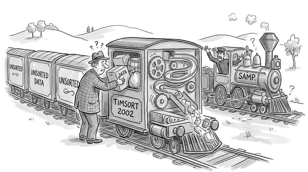
When CPython adopted Timsort (designed by Tim Peters in 2002) as the default list sorting algorithm, the decision reportedly involved a similar kind of benchmarking analysis to the pipeline described in this section. Timsort was compared against samplesort (the previous default) across multiple input distributions: random, partially sorted, reversed, and data with many duplicate keys. The property that sealed the decision was Timsort's adaptive behavior on nearly sorted data, where it achieves \(O(n)\) rather than \(O(n \log n)\), because real-world Python lists (configuration entries, database rows, log lines) are often partially ordered. The CPython benchmark suite typically uses per-distribution reporting and median aggregation, consistent with the methodology this section formalizes.
Research Frontier
The frequentist approach above (hypothesis test, \(p\)-value, reject/fail-to-reject) treats significance as binary. Bayesian performance analysis offers a richer alternative: compute the posterior probability that algorithm A is faster than algorithm B, given the observed timings. Benavoli et al. (2017) introduced Bayesian signed-rank tests for machine learning benchmarks. More recently, CodaMosa (Lemieux et al., 2023) demonstrated that LLM-guided test generation can dramatically improve code coverage for programs that traditional search-based generators struggle with, achieving up to 2x higher branch coverage on hard-to-reach code. In the benchmarking domain specifically, the EvalPlus framework (Liu et al., 2024) revealed that standard coding benchmarks like HumanEval have inadequate test suites: augmenting them with automatically generated tests reduced pass rates of GPT-4 synthesized code by 15 to 20 percentage points, exposing correctness bugs that the original benchmarks missed. These developments push in complementary directions: CodaMosa strengthens the testing side of the synthesis pipeline, while EvalPlus shows that even widely used benchmarks need the same rigor this section applies to algorithm comparison.
6. Putting It Together: The Benchmark Report
Correcting for multiple comparisons ensures that your statistical conclusions are trustworthy; the final step is packaging those conclusions, along with every measurement and caveat, into a structured report that makes the algorithm selection decision auditable and reproducible.
A complete benchmark report packages problem specification, candidate algorithms with complexity profiles (from Section 15.1), correctness verification results, timing and memory distributions with confidence intervals, statistical comparisons with effect sizes, and a final recommendation with caveats into one auditable document.
"""
Structured benchmark report that combines correctness verification,
timing, memory, and statistical comparison into one artifact.
"""
from dataclasses import dataclass, field
from datetime import datetime
import json
import platform

@dataclass
class BenchmarkReport:
    """A complete, auditable benchmark report."""
    problem: str
    created: str = field(default_factory=lambda: datetime.now().isoformat())
    environment: dict = field(default_factory=lambda: {
        "python": platform.python_version(),
        "os": platform.platform(),
        "cpu": platform.processor(),
    })
    candidates: list[dict] = field(default_factory=list)
    correctness: dict = field(default_factory=dict)
    timing_results: list[dict] = field(default_factory=list)
    memory_results: list[dict] = field(default_factory=list)
    comparisons: list[dict] = field(default_factory=list)
    winner: str = ""
    caveats: list[str] = field(default_factory=list)

    def to_json(self) -> str:
        return json.dumps(self.__dict__, indent=2, default=str)

    def summary(self) -> str:
        lines = [
            f"Benchmark Report: {self.problem}",
            f"Date: {self.created}",
            f"Environment: {self.environment['python']} on {self.environment['os']}",
            f"Candidates: {len(self.candidates)}",
            f"Winner: {self.winner or 'No clear winner'}",
        ]
        if self.caveats:
            lines.append("Caveats:")
            for c in self.caveats:
                lines.append(f"  - {c}")
        return "\n".join(lines)

# Example usage
report = BenchmarkReport(
    problem="k-nearest neighbors for 10k records in 50 dimensions",
    candidates=[
        {"name": "brute_numpy", "complexity": "O(n*d)", "correctness": "exact"},
        {"name": "kdtree_scipy", "complexity": "O(n log n)", "correctness": "exact"},
        {"name": "lsh_simple", "complexity": "O(n*L*k)", "correctness": "approximate"},
    ],
    winner="kdtree_scipy",
    caveats=[
        "KD-tree advantage diminishes above d=20 due to curse of dimensionality",
        "LSH was not tuned for recall; production deployment requires recall calibration",
        "Benchmarks run on a single machine; results may differ on other hardware",
    ],
)
print(report.summary())
A research team benchmarked five sorting algorithms and found that a novel cache-oblivious merge sort was 40% faster than all alternatives. They deployed it to production, where it promptly failed: the algorithm required \(O(n)\) auxiliary space, and the production server had 2 GB of RAM serving 1000 concurrent requests. The "winner" consumed the entire heap in under a minute. Their benchmark report had no memory column. The Algorithm Benchmark pipeline in Section 15.3 always measures both time and space, because the fastest algorithm you cannot run is not fast at all.
Try It: Benchmark Two Sorting Algorithms End to End
Complete this mini-project to practice the full synthesis, verification, and benchmarking pipeline using only Python's standard library and NumPy.
- Synthesize two candidates. Implement merge sort and heap sort in pure Python (no calls to
sorted()). Each function should accept a list of integers and return a new sorted list. - Write three Hypothesis properties. Install Hypothesis (
pip install hypothesis) and define properties: (a) the output length equals the input length, (b) the output is sorted (every element is less than or equal to the next), and (c) the output is a permutation of the input (same elements, same counts). Run both implementations against all three properties withmax_examples=200. - Benchmark on three input distributions. Using the
benchmark_algorithmharness from this section, time both algorithms on random, already-sorted, and reverse-sorted lists of size 5,000 with 50 repetitions each. Record the six median times. - Compare statistically. For each input distribution, run a Mann-Whitney U test (via
scipy.stats.mannwhitneyu) comparing the two algorithms' timing arrays. Report the \(p\)-value and the rank-biserial effect size. Apply Bonferroni correction since you are running three comparisons (\(\alpha = 0.05 / 3\)). - Write a one-paragraph verdict. State which algorithm wins on which distributions, whether any differences are practically meaningful (effect size), and note any caveats (for example, that pure-Python implementations do not reflect the relative performance of C-level library implementations).
Exercises
- Conceptual: Explain why the Mann-Whitney U test is preferred over the Student's \(t\)-test for benchmark data. Generate 1000 samples from a log-normal distribution (which models typical timing data) and show that the Shapiro-Wilk normality test rejects normality. Connect this to the broader discussion of distributional assumptions in Chapter 32.
-
Coding: Write property-based tests (using Hypothesis) for a binary search
function. Define at least three properties: (1) if the target is in the array, the
returned index contains the target; (2) if the target is not in the array, the function
returns -1; (3) the function agrees with a brute-force linear search on all inputs.
Use
st.lists(st.integers(), min_size=0, max_size=100).map(sorted)to generate sorted input arrays. -
Analysis: Benchmark Python's
dict(hash map) vs.sortedcontainers.SortedDict(balanced tree) for mixed workloads of lookups and insertions. Vary the lookup-to-insertion ratio from 99:1 to 50:50 and plot the crossover point. Use thecompare_algorithmsfunction from this section to determine at which ratio the tree becomes competitive. Report effect sizes and confidence intervals for each ratio.
Lab: Property-Based Fuzzing Catches What Unit Tests Miss
Goal: Experience firsthand how property-based testing exposes bugs that hand-written unit tests overlook, by deliberately introducing subtle defects into a search algorithm and measuring detection rates.
Tools needed: Python 3.9+, hypothesis (pip install hypothesis),
and matplotlib for plotting.
Procedure (20 minutes): (1) Implement a correct binary_search(arr, target)
that returns the index of target in sorted list arr, or -1 if absent.
(2) Create five mutant variants, each with one subtle bug: off-by-one in the loop bound,
using < instead of <=, integer overflow in midpoint calculation
((lo + hi) // 2 instead of lo + (hi - lo) // 2), wrong return
value when the array has length 1, and skipping the last element.
(3) Write a suite of 10 hand-crafted unit tests (typical cases: empty array, single element,
target at start/middle/end, target absent). Run all five mutants against these tests and
record how many mutants each test catches.
(4) Write three Hypothesis properties (result index contains target, agreement with linear
scan, correct -1 on absent targets) with max_examples=200. Run all five mutants
and record detection counts.
What to vary: Change max_examples from 10 to 500 and plot the
detection rate (fraction of mutants caught) against the number of examples. Also try
narrowing the integer range in your strategies to see how input domain affects detection.
What to observe: Property-based tests should catch all five mutants, while the
hand-written suite likely misses one or two. The detection-rate curve should flatten
around 50 to 100 examples, showing diminishing returns beyond that point. This
demonstrates why the section recommends max_examples=100 as a practical default.
What's Next
Section 15.3: Building an Algorithm Benchmark assembles the components from Sections 15.1 and 15.2 into a complete, end-to-end pipeline. You will propose three algorithm candidates for a real problem, synthesize and verify their implementations, benchmark them under controlled conditions, and select the winner with full statistical evidence. The pipeline becomes a reusable component of the Discovery Workbench.