15.3 Building an Algorithm Benchmark

1. The Pipeline Architecture

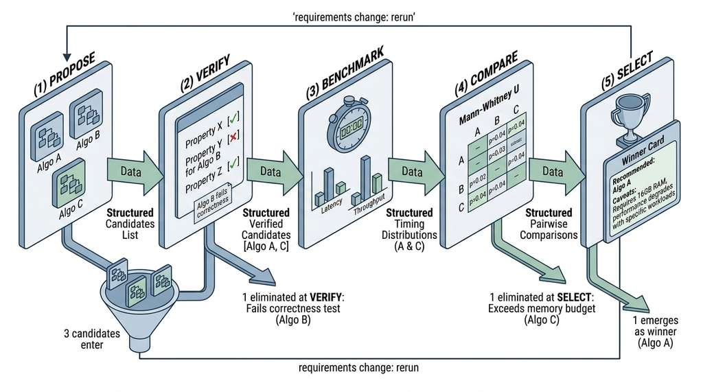
Which of three candidate algorithms should handle your production workload: the one that is provably correct but slow, the one that is fast but approximate, or the one whose performance hinges entirely on data distribution? Most teams settle this question with a quick notebook timing test and an educated guess. The five-stage pipeline replaces that guess with a process that mirrors the scientific method. Each stage maps to a scientific step: formulate hypotheses (propose candidates), design experiments (build benchmarks), collect data (run measurements), analyze results (statistical tests), and draw conclusions (select winner). This parallel is deliberate; algorithm selection is itself a form of empirical inquiry, as discussed in Chapter 2. Figure 15.3 illustrates this five-stage flow, showing how each stage consumes the previous stage's output and narrows the candidate set toward a single, statistically grounded recommendation.

Translating that scientific framing into software requires a precise data model that captures candidates, experimental conditions, and results in a single structure capable of flowing through each stage and serializing for later audit.

Choosing the wrong algorithm for a production workload can mean the difference between a query that completes in milliseconds and one that times out, silently dropping results. Teams that skip rigorous benchmarking often discover this gap only after deployment, when the cost of switching is highest.

An algorithm benchmark pipeline takes a problem specification, generates candidate solutions, verifies each for correctness, measures performance under controlled conditions, and outputs a statistically grounded recommendation. Manual selection ("I tried it and it felt faster") is neither reproducible nor defensible; a pipeline replaces subjective impressions with quantified evidence and explicit caveats. The mechanism: all candidates share a uniform function signature, the harness runs identical inputs through each, collects timing distributions, and applies nonparametric tests to distinguish real differences from noise. Use this approach when two or more viable candidates exist and the cost of choosing wrong is nontrivial. For problems with a single textbook solution, a quick notebook timing comparison suffices. In short: if you cannot rerun your algorithm selection with one command, you do not have a selection process; you have an opinion. Figure 15.3.1 illustrates the five-stage algorithm benchmark pipeline architecture.

"""
Algorithm Benchmark Pipeline: five-stage architecture
for systematic algorithm selection.
"""
from dataclasses import dataclass, field
from typing import Callable, Any, Optional
from enum import Enum
import json

class PipelineStage(Enum):
    PROPOSE = "propose"
    VERIFY = "verify"
    BENCHMARK = "benchmark"
    COMPARE = "compare"
    SELECT = "select"

@dataclass
class AlgorithmCandidate:
    """A candidate algorithm with its implementation and metadata."""
    name: str
    description: str
    complexity_time: str
    complexity_space: str
    correctness_type: str         # "exact" or "approximate"
    implementation: Callable      # the actual function
    properties_passed: bool = False
    timing_results: Optional[Any] = None
    memory_mb: float = 0.0

@dataclass
class PipelineConfig:
    """Configuration for the benchmark pipeline."""
    problem_description: str
    input_sizes: list[int] = field(default_factory=lambda: [100, 1000, 10_000])
    input_distributions: list[str] = field(default_factory=lambda: ["random", "sorted", "adversarial"])
    warmup_iterations: int = 5
    benchmark_repetitions: int = 100
    significance_level: float = 0.05
    min_effect_size: float = 0.1     # minimum meaningful rank-biserial correlation (defined in Stage 4)
    memory_budget_mb: float = 1024.0  # 1 GB default

@dataclass
class PipelineResult:
    """Complete result from the benchmark pipeline."""
    config: PipelineConfig
    candidates: list[AlgorithmCandidate]
    comparisons: list[dict]
    winner: Optional[str]
    recommendation: str
    caveats: list[str]

    def to_json(self) -> str:
        """Serialize for the Discovery Workbench."""
        return json.dumps({
            "problem": self.config.problem_description,
            "candidates": [
                {
                    "name": c.name,
                    "complexity_time": c.complexity_time,
                    "complexity_space": c.complexity_space,
                    "correctness": c.correctness_type,
                    "properties_passed": c.properties_passed,
                    "memory_mb": c.memory_mb,
                }
                for c in self.candidates
            ],
            "winner": self.winner,
            "recommendation": self.recommendation,
            "caveats": self.caveats,
        }, indent=2)

2. Stage 1: Propose Candidates

The first stage generates algorithm candidates for the problem. The stage applies the systematic enumeration from Section 15.1, producing at least three candidates from different design paradigms. For our running example (finding duplicate records by similarity), we propose brute-force cosine similarity (where cosine similarity measures the angular closeness of two vectors, yielding a value from -1 for opposite directions to 1 for identical directions), sorted-projection indexing, and locality-sensitive hashing (LSH).

"""
Stage 1: Propose three algorithm candidates for
duplicate detection by cosine similarity.
"""
import numpy as np
from typing import List, Tuple, Set

# Type alias for the function signature all candidates must share
# Input: (data matrix, similarity threshold) -> set of (i, j) pairs
DuplicateFinder = Callable[[np.ndarray, float], Set[Tuple[int, int]]]

def propose_brute_force() -> AlgorithmCandidate:
    """Candidate 1: pairwise cosine similarity via matrix multiplication."""

    def find_duplicates_brute(data: np.ndarray, threshold: float) -> Set[Tuple[int, int]]:
        # Normalize rows to unit vectors
        norms = np.linalg.norm(data, axis=1, keepdims=True)
        norms[norms == 0] = 1.0  # avoid division by zero
        normalized = data / norms
        # Cosine similarity matrix via dot product
        sim_matrix = normalized @ normalized.T
        # Extract pairs above threshold (upper triangle only)
        pairs = set()
        n = data.shape[0]
        for i in range(n):
            for j in range(i + 1, n):
                if sim_matrix[i, j] >= threshold:
                    pairs.add((i, j))
        return pairs

    return AlgorithmCandidate(
        name="brute_force_cosine",
        description="Full pairwise cosine similarity via matrix multiply",
        complexity_time="O(n^2 * d)",
        complexity_space="O(n^2)",
        correctness_type="exact",
        implementation=find_duplicates_brute,
    )

def propose_sorted_projection() -> AlgorithmCandidate:
    """Candidate 2: sort by random projection, scan within window."""

    def find_duplicates_sorted(data: np.ndarray, threshold: float) -> Set[Tuple[int, int]]:
        n, d = data.shape
        # Normalize
        norms = np.linalg.norm(data, axis=1, keepdims=True)
        norms[norms == 0] = 1.0
        normalized = data / norms
        # Project onto a random unit vector
        proj_vec = np.random.randn(d)
        proj_vec /= np.linalg.norm(proj_vec)
        projections = normalized @ proj_vec
        # Sort by projection value
        order = np.argsort(projections)
        sorted_data = normalized[order]
        sorted_proj = projections[order]
        # Scan with adaptive window: two points with cosine sim >= threshold
        # have projection difference <= sqrt(2(1 - threshold)), because for
        # unit vectors the squared Euclidean distance equals 2(1 - cos(theta))
        max_proj_diff = np.sqrt(2 * (1 - threshold)) + 0.01  # small margin
        pairs = set()
        for i in range(n):
            j = i + 1
            while j < n and (sorted_proj[j] - sorted_proj[i]) <= max_proj_diff:
                cos_sim = float(sorted_data[i] @ sorted_data[j])
                if cos_sim >= threshold:
                    # Map back to original indices
                    orig_i, orig_j = int(order[i]), int(order[j])
                    pairs.add((min(orig_i, orig_j), max(orig_i, orig_j)))
                j += 1
        return pairs

    return AlgorithmCandidate(
        name="sorted_projection",
        description="Sort by random projection, scan within distance window",
        complexity_time="O(n log n + n * w * d)",
        complexity_space="O(n)",
        correctness_type="exact",
        implementation=find_duplicates_sorted,
    )

def propose_lsh() -> AlgorithmCandidate:
    """Candidate 3: locality-sensitive hashing with random hyperplanes."""

    def find_duplicates_lsh(
        data: np.ndarray, threshold: float,
        n_bits: int = 12, n_tables: int = 6,
    ) -> Set[Tuple[int, int]]:
        n, d = data.shape
        norms = np.linalg.norm(data, axis=1, keepdims=True)
        norms[norms == 0] = 1.0
        normalized = data / norms
        pairs = set()
        for _ in range(n_tables):
            # Random hyperplane hashing
            planes = np.random.randn(n_bits, d)
            hashes = (normalized @ planes.T > 0)
            # Convert boolean rows to integer hash keys
            # Pack each row of booleans into a compact byte array serving as the hash key
            hash_keys = np.packbits(hashes, axis=1, bitorder="little")
            # Group by hash bucket
            buckets: dict[bytes, list[int]] = {}
            for idx in range(n):
                key = hash_keys[idx].tobytes()
                buckets.setdefault(key, []).append(idx)
            # Compare within buckets
            for bucket in buckets.values():
                if len(bucket) > 1 and len(bucket) < 200:  # skip very large buckets
                    for bi in range(len(bucket)):
                        for bj in range(bi + 1, len(bucket)):
                            ii, jj = bucket[bi], bucket[bj]
                            cos_sim = float(normalized[ii] @ normalized[jj])
                            if cos_sim >= threshold:
                                pairs.add((min(ii, jj), max(ii, jj)))
        return pairs

    return AlgorithmCandidate(
        name="lsh_hyperplane",
        description="Locality-sensitive hashing with random hyperplane projections",
        complexity_time="O(n * L * k + n * b * d)",
        complexity_space="O(n * L)",
        correctness_type="approximate",
        implementation=find_duplicates_lsh,
    )

# Propose all three
candidates = [propose_brute_force(), propose_sorted_projection(), propose_lsh()]
for c in candidates:
    print(f"Proposed: {c.name} ({c.correctness_type})")
    print(f"  Time: {c.complexity_time}, Space: {c.complexity_space}")
    print(f"  {c.description}\n")

3. Stage 2: Verify Correctness

Before benchmarking, every candidate must pass correctness verification. A fast but wrong algorithm is useless (and dangerous, because its speed creates confidence in incorrect results). The verification uses property-based testing, where the test framework generates random inputs and checks that specified invariants hold for every generated case, following the pattern from Section 15.2.

"""
Stage 2: Verify correctness using property-based testing.
Properties for duplicate-detection algorithms.
"""
from hypothesis import given, settings, HealthCheck
from hypothesis import strategies as st
import numpy as np

def verify_duplicate_finder(
    impl: Callable[[np.ndarray, float], set[tuple[int, int]]],
    name: str,
    is_approximate: bool = False,
) -> bool:
    """Verify a duplicate-finder implementation against correctness properties."""
    errors = []

    # Property 1: Symmetry. If (i, j) is found, (j, i) should not also appear
    # (we canonicalize to i < j)
    @given(n=st.integers(min_value=3, max_value=50),
           d=st.integers(min_value=2, max_value=10))
    @settings(max_examples=50, suppress_health_check=[HealthCheck.too_slow])
    def prop_canonical_pairs(n, d):
        data = np.random.randn(n, d)
        pairs = impl(data, 0.5)
        for i, j in pairs:
            assert i < j, f"Non-canonical pair: ({i}, {j})"

    # Property 2: Self-similarity excluded. No (i, i) pairs.
    @given(n=st.integers(min_value=3, max_value=50),
           d=st.integers(min_value=2, max_value=10))
    @settings(max_examples=50, suppress_health_check=[HealthCheck.too_slow])
    def prop_no_self_pairs(n, d):
        data = np.random.randn(n, d)
        pairs = impl(data, 0.5)
        for i, j in pairs:
            assert i != j, f"Self-pair: ({i}, {j})"

    # Property 3: Identical vectors produce a pair (threshold <= 1.0)
    @given(d=st.integers(min_value=2, max_value=10))
    @settings(max_examples=30, suppress_health_check=[HealthCheck.too_slow])
    def prop_identical_detected(d):
        vec = np.random.randn(d)
        data = np.vstack([vec, vec, np.random.randn(d)])  # first two identical
        pairs = impl(data, 0.99)
        if not is_approximate:
            assert (0, 1) in pairs, "Identical vectors not detected as duplicates"

    # Property 4: Orthogonal vectors excluded (cos sim = 0, threshold > 0)
    @given(st.integers(min_value=2, max_value=5))
    @settings(max_examples=30, suppress_health_check=[HealthCheck.too_slow])
    def prop_orthogonal_excluded(d):
        # Construct two orthogonal vectors
        v1 = np.zeros(max(d, 2))
        v1[0] = 1.0
        v2 = np.zeros(max(d, 2))
        v2[1] = 1.0
        data = np.vstack([v1, v2])
        pairs = impl(data, 0.5)
        assert (0, 1) not in pairs, "Orthogonal vectors incorrectly marked as duplicates"

    # Property 5: Agreement with brute force (reference oracle)
    @given(n=st.integers(min_value=3, max_value=30),
           d=st.integers(min_value=2, max_value=5))
    @settings(max_examples=30, suppress_health_check=[HealthCheck.too_slow])
    def prop_agrees_with_oracle(n, d):
        data = np.random.randn(n, d)
        threshold = 0.7
        # Oracle: brute force
        norms = np.linalg.norm(data, axis=1, keepdims=True)
        norms[norms == 0] = 1.0
        normed = data / norms
        oracle_pairs = set()
        for i in range(n):
            for j in range(i + 1, n):
                if float(normed[i] @ normed[j]) >= threshold:
                    oracle_pairs.add((i, j))
        impl_pairs = impl(data, threshold)
        if not is_approximate:
            assert impl_pairs == oracle_pairs, (
                f"Mismatch: impl found {impl_pairs - oracle_pairs} extra, "
                f"missed {oracle_pairs - impl_pairs}"
            )
        else:
            # Approximate: check recall >= 30% (lenient for random hyperplane LSH)
            if len(oracle_pairs) > 0:
                recall = len(impl_pairs & oracle_pairs) / len(oracle_pairs)
                assert recall >= 0.3, f"Recall too low: {recall:.2f}"

    properties = [
        ("canonical_pairs", prop_canonical_pairs),
        ("no_self_pairs", prop_no_self_pairs),
        ("identical_detected", prop_identical_detected),
        ("orthogonal_excluded", prop_orthogonal_excluded),
        ("agrees_with_oracle", prop_agrees_with_oracle),
    ]

    for prop_name, prop_fn in properties:
        try:
            prop_fn()
            print(f"  [{name}] PASS: {prop_name}")
        except Exception as e:
            print(f"  [{name}] FAIL: {prop_name}: {e}")
            errors.append(prop_name)

    passed = len(errors) == 0
    return passed

# Verify all candidates
for candidate in candidates:
    print(f"\nVerifying {candidate.name}:")
    candidate.properties_passed = verify_duplicate_finder(
        candidate.implementation,
        candidate.name,
        is_approximate=(candidate.correctness_type == "approximate"),
    )
    status = "PASSED" if candidate.properties_passed else "FAILED"
    print(f"  Overall: {status}")

4. Stage 3: Benchmark Performance

With correctness verified, the pipeline measures performance. The benchmark runs each candidate across multiple input sizes and distributions, collecting timing and memory measurements with the methodology from Section 15.2. (At \(n = 10{,}000\), the ratio of \(n^2\) to \(n \log n\) exceeds 750; that single factor is why brute force takes minutes where projection-based methods finish in fractions of a second.)

"""
Stage 3: Benchmark all verified candidates across
input sizes and distributions.
"""
import timeit
import gc
import tracemalloc
import statistics
import numpy as np
from dataclasses import dataclass
from typing import Callable

@dataclass
class BenchmarkResult:
    """Timing and memory results for one (algorithm, size, distribution) triple."""
    algorithm: str
    input_size: int
    distribution: str
    timings_ms: list[float]
    median_ms: float = 0.0
    iqr_ms: float = 0.0
    peak_memory_mb: float = 0.0

    def __post_init__(self):
        if self.timings_ms:
            self.median_ms = statistics.median(self.timings_ms)
            q1 = np.percentile(self.timings_ms, 25)
            q3 = np.percentile(self.timings_ms, 75)
            self.iqr_ms = q3 - q1

def generate_input(n: int, d: int, distribution: str) -> np.ndarray:
    """Generate input data for a given distribution."""
    if distribution == "random":
        return np.random.randn(n, d)
    elif distribution == "clustered":
        # 5 clusters with Gaussian noise
        centers = np.random.randn(5, d) * 10
        labels = np.random.randint(0, 5, size=n)
        return centers[labels] + np.random.randn(n, d) * 0.5
    elif distribution == "adversarial":
        # All vectors nearly identical (maximizes pairs found)
        base = np.random.randn(d)
        return np.tile(base, (n, 1)) + np.random.randn(n, d) * 0.01
    else:
        return np.random.randn(n, d)

def run_benchmarks(
    candidates: list[AlgorithmCandidate],
    config: PipelineConfig,
    d: int = 50,
    threshold: float = 0.9,
) -> list[BenchmarkResult]:
    """Run benchmarks for all verified candidates."""
    results = []
    verified = [c for c in candidates if c.properties_passed]
    print(f"Benchmarking {len(verified)} verified candidates "
          f"across {len(config.input_sizes)} sizes x "
          f"{len(config.input_distributions)} distributions\n")

    for candidate in verified:
        for n in config.input_sizes:
            for dist in config.input_distributions:
                print(f"  {candidate.name} | n={n:,} | {dist}...", end=" ")

                # Warmup
                for _ in range(config.warmup_iterations):
                    data = generate_input(n, d, dist)
                    candidate.implementation(data, threshold)

                # Timed runs
                timings_ms = []
                for _ in range(config.benchmark_repetitions):
                    data = generate_input(n, d, dist)
                    gc.disable()  # prevent GC pauses from inflating timings
                    start = timeit.default_timer()
                    candidate.implementation(data, threshold)
                    elapsed = timeit.default_timer() - start
                    gc.enable()
                    timings_ms.append(elapsed * 1000)

                # Memory measurement (separate pass, fewer repetitions)
                data = generate_input(n, d, dist)
                tracemalloc.start()
                candidate.implementation(data, threshold)
                _, peak = tracemalloc.get_traced_memory()
                tracemalloc.stop()
                peak_mb = peak / (1024 * 1024)

                result = BenchmarkResult(
                    algorithm=candidate.name,
                    input_size=n,
                    distribution=dist,
                    timings_ms=timings_ms,
                    peak_memory_mb=peak_mb,
                )
                results.append(result)
                print(f"median={result.median_ms:.2f}ms, "
                      f"IQR={result.iqr_ms:.2f}ms, "
                      f"mem={peak_mb:.1f}MB")

    return results

# Configure and run
config = PipelineConfig(
    problem_description="Duplicate detection by cosine similarity in literature embeddings",
    input_sizes=[100, 500, 2000],
    input_distributions=["random", "clustered", "adversarial"],
    warmup_iterations=3,
    benchmark_repetitions=50,
    significance_level=0.05,
    memory_budget_mb=512.0,
)

# benchmark_results = run_benchmarks(candidates, config)

Building a benchmark is not just writing a timing loop; it requires defending the measurements against threats to validity. The warmup iterations above allow CPU caches and (in JIT-compiled runtimes) the compiler to reach steady state. Disabling garbage collection during each timed call prevents GC pauses from appearing as algorithm slowdowns. Measuring memory in a separate pass avoids the overhead of tracemalloc distorting the timing results. Beyond these code-level precautions, be aware of system-level noise: background processes, CPU frequency scaling, and thermal throttling can all shift timing distributions. Running benchmarks on an otherwise idle machine and reporting the interquartile range (as this harness does) rather than the mean helps surface these effects.

5. Stage 4: Statistical Comparison

With timing data collected, the next stage compares algorithms pairwise using the Mann-Whitney U test (a nonparametric statistical test that compares two independent samples without assuming normal distributions) with Bonferroni correction (which divides the significance threshold by the number of comparisons to control the family-wise false-positive rate), following Section 15.2. Each comparison runs separately per input size and distribution, because an algorithm that wins on random data may lose on adversarial data.

"""
Stage 4: Statistical comparison of all candidate pairs
per input size and distribution.
"""
from scipy import stats
from itertools import combinations

@dataclass
class PairwiseComparison:
    """Result of comparing two algorithms on one (size, distribution)."""
    algo_a: str
    algo_b: str
    input_size: int
    distribution: str
    median_a_ms: float
    median_b_ms: float
    u_statistic: float
    p_value: float
    effect_size: float     # rank-biserial correlation
    significant: bool
    faster: str

def statistical_comparison(
    results: list[BenchmarkResult],
    alpha: float = 0.05,
) -> list[PairwiseComparison]:
    """Compare all algorithm pairs per (size, distribution) with Bonferroni."""
    # Group results by (size, distribution)
    grouped: dict[tuple[int, str], list[BenchmarkResult]] = {}
    for r in results:
        key = (r.input_size, r.distribution)
        grouped.setdefault(key, []).append(r)

    all_comparisons = []
    for (size, dist), group in sorted(grouped.items()):
        n_pairs = len(group) * (len(group) - 1) // 2
        corrected_alpha = alpha / max(n_pairs, 1)

        print(f"\n--- n={size:,}, distribution={dist} "
              f"(Bonferroni alpha={corrected_alpha:.4f}) ---")

        for a, b in combinations(group, 2):
            ta = np.array(a.timings_ms)
            tb = np.array(b.timings_ms)
            u_stat, p_val = stats.mannwhitneyu(ta, tb, alternative="two-sided")

            # Rank-biserial effect size
            n1, n2 = len(ta), len(tb)
            effect = 1 - (2 * u_stat) / (n1 * n2)

            sig = p_val < corrected_alpha
            faster = a.algorithm if np.median(ta) < np.median(tb) else b.algorithm

            comp = PairwiseComparison(
                algo_a=a.algorithm,
                algo_b=b.algorithm,
                input_size=size,
                distribution=dist,
                median_a_ms=float(np.median(ta)),
                median_b_ms=float(np.median(tb)),
                u_statistic=u_stat,
                p_value=p_val,
                effect_size=effect,
                significant=sig,
                faster=faster,
            )
            all_comparisons.append(comp)

            sig_marker = "*" if sig else " "
            print(f"  {a.algorithm} vs {b.algorithm}: "
                  f"p={p_val:.4f}{sig_marker} | "
                  f"effect={effect:+.3f} | "
                  f"faster={faster}")

    return all_comparisons

Step-Through: Bonferroni-Corrected Pairwise Comparison

Trace through Stage 4 with three algorithms (A, B, C) at one input size and one distribution. We have three pairwise comparisons, so the Bonferroni-corrected significance level is \(\alpha_{\text{corrected}} = 0.05 / 3 = 0.0167\).

Pair 1: A vs B. Median times: A = 12.3 ms, B = 18.7 ms. Mann-Whitney U = 342, \(p = 0.0003\). Since \(0.0003 < 0.0167\), this is significant. Winner: A. Rank-biserial effect size: \(r = 1 - 2(342)/(50 \times 50) = 0.727\) (large effect).

Pair 2: A vs C. Median times: A = 12.3 ms, C = 13.1 ms. Mann-Whitney U = 1180, \(p = 0.42\). Since \(0.42 > 0.0167\), this is not significant. No winner declared. Effect size: \(r = 0.056\) (negligible).

Pair 3: B vs C. Median times: B = 18.7 ms, C = 13.1 ms. Mann-Whitney U = 485, \(p = 0.0021\). Since \(0.0021 < 0.0167\), this is significant. Winner: C. Effect size: \(r = 0.612\) (large).

Scoreboard: A has 1 win, 0 losses (score +1). B has 0 wins, 2 losses (score \(-2\)). C has 1 win, 0 losses (score +1). A and C are tied. The tiebreaker checks median time at the largest input size. If A is faster there, A wins overall. Notice that the Bonferroni correction prevented us from declaring A significantly faster than C on a \(p = 0.42\) result that would have failed even without correction; on tighter margins (say \(p = 0.03\)), the correction would matter.

6. Stage 5: Select the Winner

The final stage synthesizes all comparisons into a recommendation. The selection logic must handle nuance: an algorithm might win on large inputs but lose on small ones, or win on random data but lose on adversarial data. The recommendation should account for the user's specific constraints (input size range, expected distribution, memory budget).

"""
Stage 5: Select the winner based on statistical comparisons,
memory constraints, and user priorities.
"""

def select_winner(
    candidates: list[AlgorithmCandidate],
    comparisons: list[PairwiseComparison],
    config: PipelineConfig,
    benchmark_results: list[BenchmarkResult],
) -> PipelineResult:
    """
    Select the winning algorithm based on:
    1. Correctness (must pass all properties)
    2. Memory budget (must fit within budget)
    3. Statistical dominance (wins most comparisons)
    """
    verified = [c for c in candidates if c.properties_passed]

    # Filter by memory budget
    memory_usage = {}
    for r in benchmark_results:
        key = r.algorithm
        memory_usage[key] = max(memory_usage.get(key, 0), r.peak_memory_mb)

    within_budget = [
        c for c in verified
        if memory_usage.get(c.name, 0) <= config.memory_budget_mb
    ]

    caveats = []
    excluded_memory = set(c.name for c in verified) - set(c.name for c in within_budget)
    if excluded_memory:
        caveats.append(
            f"Excluded for exceeding {config.memory_budget_mb}MB memory budget: "
            f"{', '.join(excluded_memory)}"
        )

    if not within_budget:
        return PipelineResult(
            config=config,
            candidates=candidates,
            comparisons=[],
            winner=None,
            recommendation="No candidate fits within the memory budget.",
            caveats=caveats,
        )

    # Count significant wins per algorithm across all conditions
    win_counts: dict[str, int] = {c.name: 0 for c in within_budget}
    loss_counts: dict[str, int] = {c.name: 0 for c in within_budget}
    total_comparisons_per_algo: dict[str, int] = {c.name: 0 for c in within_budget}

    valid_names = set(c.name for c in within_budget)
    for comp in comparisons:
        if comp.algo_a in valid_names and comp.algo_b in valid_names:
            total_comparisons_per_algo[comp.algo_a] = (
                total_comparisons_per_algo.get(comp.algo_a, 0) + 1
            )
            total_comparisons_per_algo[comp.algo_b] = (
                total_comparisons_per_algo.get(comp.algo_b, 0) + 1
            )
            if comp.significant:
                win_counts[comp.faster] = win_counts.get(comp.faster, 0) + 1
                loser = comp.algo_b if comp.faster == comp.algo_a else comp.algo_a
                loss_counts[loser] = loss_counts.get(loser, 0) + 1

    # Score: wins minus losses
    scores = {
        name: win_counts.get(name, 0) - loss_counts.get(name, 0)
        for name in valid_names
    }
    best_name = max(scores, key=scores.get)
    best_score = scores[best_name]

    # Check for ties
    tied = [name for name, s in scores.items() if s == best_score]
    if len(tied) > 1:
        # Break tie by median time at largest input size
        largest_n = max(config.input_sizes)
        median_at_largest = {}
        for r in benchmark_results:
            if r.algorithm in tied and r.input_size == largest_n:
                median_at_largest.setdefault(r.algorithm, []).append(r.median_ms)
        avg_median = {
            name: np.mean(medians)
            for name, medians in median_at_largest.items()
        }
        if avg_median:
            best_name = min(avg_median, key=avg_median.get)
        caveats.append(
            f"Tie broken by median time at n={largest_n:,}: "
            f"{', '.join(f'{n}={avg_median.get(n, 0):.2f}ms' for n in tied)}"
        )

    # Build recommendation
    winner_candidate = next(c for c in within_budget if c.name == best_name)
    recommendation = (
        f"Recommended: {best_name} "
        f"(time: {winner_candidate.complexity_time}, "
        f"space: {winner_candidate.complexity_space}, "
        f"correctness: {winner_candidate.correctness_type}). "
        f"Won {win_counts.get(best_name, 0)} of "
        f"{total_comparisons_per_algo.get(best_name, 0)} comparisons "
        f"at alpha={config.significance_level}."
    )

    # Add distribution-specific caveats
    for dist in config.input_distributions:
        dist_comps = [c for c in comparisons if c.distribution == dist and c.significant]
        dist_winners = set(c.faster for c in dist_comps)
        if dist_winners and best_name not in dist_winners:
            actual_winner = dist_winners.pop()
            caveats.append(
                f"On {dist} data, {actual_winner} outperforms {best_name}."
            )

    return PipelineResult(
        config=config,
        candidates=candidates,
        comparisons=[{
            "algo_a": c.algo_a, "algo_b": c.algo_b,
            "size": c.input_size, "dist": c.distribution,
            "p_value": c.p_value, "effect": c.effect_size,
            "faster": c.faster, "significant": c.significant,
        } for c in comparisons],
        winner=best_name,
        recommendation=recommendation,
        caveats=caveats,
    )

7. The Complete Pipeline

All five stages assemble into a single callable pipeline. The pipeline function takes a configuration and a list of candidate factories, runs all stages in sequence, and produces a complete, serializable result. As shown in Figure 15.3, the output feeds back into subsequent pipeline runs when requirements evolve.

"""
The complete Algorithm Benchmark pipeline:
propose -> verify -> benchmark -> compare -> select.
"""

def run_algorithm_benchmark(
    candidate_factories: list[Callable[[], AlgorithmCandidate]],
    config: PipelineConfig,
    d: int = 50,
    threshold: float = 0.9,
) -> PipelineResult:
    """
    End-to-end algorithm benchmark pipeline.

    Args:
        candidate_factories: Functions that create algorithm candidates.
        config: Pipeline configuration (sizes, distributions, thresholds).
        d: Dimensionality of input data.
        threshold: Similarity threshold for duplicate detection.

    Returns:
        PipelineResult with winner, comparisons, and caveats.
    """
    print("=" * 60)
    print(f"Algorithm Benchmark: {config.problem_description}")
    print("=" * 60)

    # Stage 1: Propose
    print("\n[Stage 1] Proposing candidates...")
    candidates = [factory() for factory in candidate_factories]
    for c in candidates:
        print(f"  {c.name}: {c.description}")

    # Stage 2: Verify
    print("\n[Stage 2] Verifying correctness...")
    for c in candidates:
        print(f"\n  Verifying {c.name}:")
        c.properties_passed = verify_duplicate_finder(
            c.implementation, c.name,
            is_approximate=(c.correctness_type == "approximate"),
        )
        status = "PASSED" if c.properties_passed else "FAILED"
        print(f"  Result: {status}")

    verified = [c for c in candidates if c.properties_passed]
    if len(verified) < 2:
        print(f"\nOnly {len(verified)} candidates passed verification. "
              f"Need at least 2 for comparison.")
        return PipelineResult(
            config=config, candidates=candidates,
            comparisons=[], winner=verified[0].name if verified else None,
            recommendation="Insufficient verified candidates for comparison.",
            caveats=["Only one candidate passed correctness verification."],
        )

    # Stage 3: Benchmark
    print("\n[Stage 3] Running benchmarks...")
    benchmark_results = run_benchmarks(verified, config, d=d, threshold=threshold)

    # Stage 4: Compare
    print("\n[Stage 4] Statistical comparison...")
    comparisons = statistical_comparison(
        benchmark_results, alpha=config.significance_level
    )

    # Stage 5: Select
    print("\n[Stage 5] Selecting winner...")
    result = select_winner(candidates, comparisons, config, benchmark_results)
    print(f"\n{'=' * 60}")
    print(f"RECOMMENDATION: {result.recommendation}")
    if result.caveats:
        print("CAVEATS:")
        for caveat in result.caveats:
            print(f"  - {caveat}")
    print(f"{'=' * 60}")

    return result

# Run the complete pipeline
# pipeline_result = run_algorithm_benchmark(
#     candidate_factories=[propose_brute_force, propose_sorted_projection, propose_lsh],
#     config=config,
# )
# print(pipeline_result.to_json())

8. Integration with the Discovery Workbench

With the pipeline assembled as a self-contained function, the remaining question is how it connects to the broader development infrastructure so that its recommendations become persistent, auditable decisions.

The Algorithm Benchmark pipeline becomes a component of the Discovery Workbench introduced in Chapter 6. It connects to three other Workbench components:

Workbench Integration Points

Architecture Decision Records (Chapter 14): Each algorithm selection produces a decision record that links the chosen algorithm to the benchmark evidence supporting it. When an Architecture Decision Record (ADR) specifies a performance requirement ("API response time under 100ms"), the benchmark report provides the evidence that the chosen algorithm meets it.

Implementation Workflows (Chapter 16): The winning algorithm's implementation becomes the starting point for AI-assisted coding. The property-based tests from Stage 2 become the correctness regression suite. The benchmark from Stage 3 becomes the performance regression suite.

Testing and QA (Chapter 18): The property-based testing patterns from Stage 2 extend into the broader testing strategy. Hypothesis strategies written for algorithm verification are reusable as fuzz-testing inputs for the production implementation.

Exercises

1. Conceptual: The pipeline uses Bonferroni correction for multiple comparisons. An alternative is the Holm-Bonferroni method, a sequential procedure that sorts the \(p\)-values from smallest to largest and applies progressively less strict thresholds, achieving higher statistical power while still controlling the family-wise error rate. Research the Holm-Bonferroni procedure and explain how it orders \(p\)-values and applies decreasing thresholds. Under what conditions would switching from Bonferroni to Holm-Bonferroni change the pipeline's winner? Relate to the hypothesis testing discussion in Chapter 2.
2. Coding: Extend the pipeline to support a fourth candidate: approximate nearest-neighbor search using Meta's FAISS library (originally developed at Facebook AI Research, now maintained under the Meta open source umbrella) (pip install faiss-cpu). Implement the candidate factory function, add it to the pipeline, and run the full benchmark. Facebook AI Similarity Search (FAISS) uses inverted file indexing with product quantization; compare its recall-vs-speed trade-off against the simple LSH candidate. Use faiss.IndexFlatIP for exact search and faiss.IndexIVFFlat for approximate search.
3. Analysis: Run the complete pipeline on your machine with input_sizes=[100, 1000, 5000, 10000] and three distributions. At which input size does the brute-force candidate become significantly slower than the alternatives? Plot the scaling behavior (input size vs. median time) for all three candidates on the same axes and annotate the crossover points. Verify that the empirical scaling matches the theoretical complexity from Section 15.1.