19.1 Hypothesis-Driven Debugging

1. Debugging as Scientific Inquiry

Your test suite passed at midnight; by morning, 47 tests are red, and the diff contains 200 changed lines across 12 files. Staring at the traceback hoping for insight is the software equivalent of a scientist squinting at a broken apparatus. The productive response, in both cases, is identical: formulate hypotheses, design experiments to distinguish between them, and iteratively narrow the set of plausible explanations until only one remains.

Studies of professional developers suggest that unstructured debugging can account for roughly half of total development time on mature codebases, and that proportion tends to grow as systems become more distributed. The cost is not just hours; random code changes introduced while hunting a bug frequently create new defects, compounding the original problem.

In hypothesis-driven debugging, the developer treats every observed failure as evidence, then generates, ranks, and tests candidate root causes instead of modifying code at random. Unstructured debugging (inserting print statements, toggling changes, and hoping something works) scales poorly. As codebases grow, the space of possible faults grows combinatorially, and ad hoc exploration wastes most of its effort on irrelevant code paths. The mechanism is straightforward: observe the symptom, enumerate plausible explanations, design the cheapest experiment that distinguishes between them, run it, eliminate the disproven hypotheses, and repeat until exactly one explanation survives. Use this approach whenever a bug resists a quick visual inspection of the traceback. For trivial typos or import errors that the traceback already pinpoints, a formal hypothesis cycle adds overhead without benefit.

The Scientific Method Correspondence

The analogy is precise: the observation is a failing test, the hypotheses are candidate root causes (a wrong conditional, an off-by-one, a missing null check), the experiments are targeted test runs that confirm or eliminate each candidate, and the conclusion is a verified patch. This cycle mirrors the scientific method covered in Chapter 2. In short: A bug is a failed hypothesis about what the code does; debugging is the experiment that reveals which hypothesis was wrong.

2. Delta Debugging: Binary Search Over Change Sets

Delta debugging, introduced by Andreas Zeller, answers a deceptively simple question: given a set of changes that caused a test to fail, what is the minimal subset of those changes that is sufficient to reproduce the failure? The answer is found through a binary search process that systematically partitions the change set and tests each partition.

2.1 The Algorithm

Let \(C = \{c_1, c_2, \ldots, c_n\}\) be a set of changes (lines modified, commits applied, configuration values altered). Define a test function \(\text{test}(S)\) that returns \(\text{FAIL}\) when the subset \(S \subseteq C\) reproduces the failure and \(\text{PASS}\) otherwise. The ddmin (delta debugging minimization) algorithm finds a 1-minimal subset \(S^* \subseteq C\) such that \(\text{test}(S^*) = \text{FAIL}\) and for every proper subset \(S' \subset S^*\), \(\text{test}(S') = \text{PASS}\). Here, 1-minimal means that removing any single element from the result causes the test to pass; the set cannot be reduced further one element at a time.

The algorithm works by repeatedly splitting the current change set into halves and testing each half. If one half alone triggers the failure, the other half is irrelevant and can be discarded. If neither half alone triggers the failure, the algorithm increases the granularity, splitting into quarters, eighths, and so on, until it finds the minimal set. The worst-case complexity is \(O(n^2)\) test executions, but the typical case for bugs caused by a small number of interacting changes is \(O(n \log n)\).

"""
Delta debugging: find the minimal failure-inducing subset of changes.
Implements the ddmin algorithm from Zeller & Hildebrandt (2002).
"""
from enum import Enum
from typing import Callable, Sequence, TypeVar

T = TypeVar("T")


class TestResult(Enum):
    PASS = "pass"
    FAIL = "fail"
    UNRESOLVED = "unresolved"


def ddmin(
    changes: Sequence[T],
    test_fn: Callable[[Sequence[T]], TestResult],
    granularity: int = 2,
) -> list[T]:
    """Find 1-minimal failure-inducing subset of changes.

    Args:
        changes: The full set of changes that causes a failure.
        test_fn: Function that returns FAIL if the subset triggers
                 the bug, PASS if it does not, UNRESOLVED otherwise.
        granularity: Initial partition count (default 2 for binary).

    Returns:
        Minimal subset that still triggers the failure.
    """
    assert test_fn(changes) == TestResult.FAIL, "Full set must fail"

    n = granularity
    current = list(changes)

    while len(current) >= 2:
        # Partition current changes into n roughly equal subsets
        chunk_size = max(1, len(current) // n)
        subsets = [
            current[i : i + chunk_size]
            for i in range(0, len(current), chunk_size)
        ]

        found_smaller = False

        # Try each subset alone
        for subset in subsets:
            if test_fn(subset) == TestResult.FAIL:
                current = subset
                n = 2
                found_smaller = True
                break

        if found_smaller:
            continue

        # Try each complement (all changes except one subset)
        for i, subset in enumerate(subsets):
            complement = []
            for j, s in enumerate(subsets):
                if j != i:
                    complement.extend(s)
            if test_fn(complement) == TestResult.FAIL:
                current = complement
                n = max(n - 1, 2)
                found_smaller = True
                break

        if not found_smaller:
            if n >= len(current):
                break  # Cannot split further; current is minimal
            n = min(n * 2, len(current))

    return current

Let us see this in action. Suppose a commit introduces 20 changed lines, and only 3 of them interact to cause a regression. Instead of manually bisecting, ddmin systematically tests subsets and finds those 3 lines in roughly \(O(20 \log 20) \approx 87\) test runs, far fewer than the \(2^{20} \approx 1{,}000{,}000\) subsets a brute-force approach would require.

"""
Demonstration: applying ddmin to isolate a failure-inducing change.
"""


def apply_changes(base_code: str, changes: list[str]) -> str:
    """Simulate applying a set of line-level changes to source code."""
    result = base_code
    for change in changes:
        result += f"\n{change}"
    return result


def simulate_test(changes: list[str]) -> TestResult:
    """A simulated test that fails when specific changes co-occur.

    The bug requires BOTH 'x = x - 1' AND 'if x > 0' to be present;
    either alone does not trigger the failure.
    """
    code = " ".join(changes)
    has_decrement = "x = x - 1" in code
    has_wrong_guard = "if x > 0" in code  # should be >= 0
    if has_decrement and has_wrong_guard:
        return TestResult.FAIL
    return TestResult.PASS


# 10 changes, only 2 of which interact to cause the bug
all_changes = [
    "y = 42",
    "x = x - 1",       # Bug component 1
    "z = compute(a)",
    "log.info('step')",
    "if x > 0",         # Bug component 2 (should be >= 0)
    "cache.clear()",
    "result.append(v)",
    "counter += 1",
    "db.commit()",
    "return result",
]

minimal = ddmin(all_changes, simulate_test)
print(f"Minimal failure set ({len(minimal)} changes): {minimal}")
# Output: Minimal failure set (2 changes): ['x = x - 1', 'if x > 0']

3. Spectrum-Based Fault Localization

Delta debugging tells you which changes caused a bug. spectrum-based fault localization (SBFL) tells you which lines of existing code are most likely at fault, given a set of passing and failing test executions. The idea is simple: a line that is executed by many failing tests and few passing tests is more suspicious than a line executed uniformly by both.

3.1 The Program Spectrum

A program spectrum is a record of which source lines were executed during a particular test run. Given \(m\) test cases \(\{t_1, t_2, \ldots, t_m\}\) and \(n\) source lines \(\{s_1, s_2, \ldots, s_n\}\), the spectrum is a binary matrix \(M\) where \(M_{ij} = 1\) if test \(t_i\) executed line \(s_j\), and \(M_{ij} = 0\) otherwise. Each test also has an outcome: pass (\(P\)) or fail (\(F\)).

For each line \(s_j\), we compute four counts from the spectrum. These counts capture how strongly the line's execution correlates with test failure:

• \(e_f(s_j)\): number of failing tests that execute line \(s_j\)
• \(e_p(s_j)\): number of passing tests that execute line \(s_j\)
• \(n_f(s_j)\): number of failing tests that do not execute line \(s_j\)
• \(n_p(s_j)\): number of passing tests that do not execute line \(s_j\)

3.2 The Ochiai Coefficient

Several suspiciousness metrics have been proposed. The Ochiai coefficient, borrowed from ecology where it measures species co-occurrence, consistently outperforms alternatives in empirical evaluations. For a source line \(s_j\):

The numerator rewards lines that appear in failing tests. The denominator penalizes lines that also appear in passing tests (low discrimination) and lines that are absent from some failing tests (incomplete coverage of failures). A line with \(\text{Ochiai} = 1.0\) appears in every failing test and no passing test; it is maximally suspicious. A line with \(\text{Ochiai} = 0.0\) never appears in a failing test; it is cleared.

Mental Model

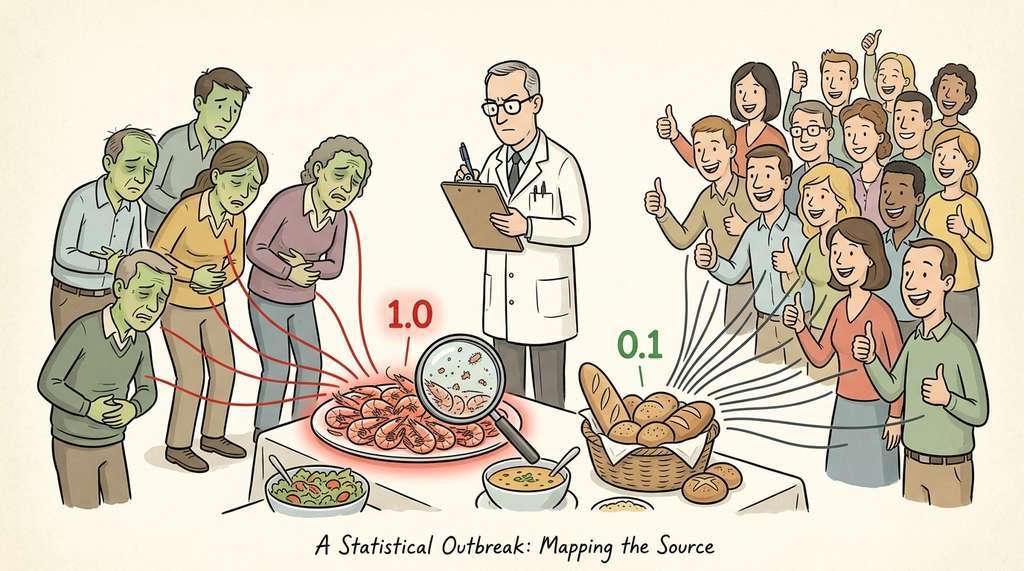
Think of the Ochiai coefficient like a food-poisoning investigation. A health inspector has reports from 20 diners: 5 got sick, 15 did not. Each report lists what the diner ate. If every sick diner ate the shrimp and none of the healthy diners did, the shrimp gets a suspiciousness score of 1.0. If both sick and healthy diners ate the bread, the bread scores low because it does not discriminate between outcomes. The Ochiai coefficient works the same way: it scores each line of code by how exclusively it co-occurs with failure, just as the inspector scores each dish by how exclusively it co-occurs with illness. The denominator penalizes "popular" dishes (lines run by many passing tests too) and rewards dishes consumed by every sick person (lines present in all failing tests).

For comparison, other metrics use the same four counts differently. The Tarantula metric normalizes by the total number of passing and failing tests:

Empirical studies by Abreu et al. (2007) show that Ochiai ranks the faulty line higher than Tarantula in 80% of cases, making it the preferred default for automated fault localization.

"""
Spectrum-based fault localization with the Ochiai coefficient.
Given a coverage matrix and test outcomes, rank lines by suspiciousness.
"""
import math
from dataclasses import dataclass


@dataclass
class SpectrumEntry:
    """Coverage and outcome data for one source line."""
    line_number: int
    source_text: str
    executed_by_failing: int   # e_f
    executed_by_passing: int   # e_p
    not_executed_failing: int  # n_f
    not_executed_passing: int  # n_p


def ochiai(entry: SpectrumEntry) -> float:
    """Compute the Ochiai suspiciousness coefficient.

    Returns a value in [0, 1] where 1.0 = maximally suspicious.
    """
    ef = entry.executed_by_failing
    ep = entry.executed_by_passing
    nf = entry.not_executed_failing

    denominator = math.sqrt((ef + nf) * (ef + ep))
    if denominator == 0:
        return 0.0
    return ef / denominator


def tarantula(entry: SpectrumEntry) -> float:
    """Compute the Tarantula suspiciousness metric for comparison."""
    ef = entry.executed_by_failing
    ep = entry.executed_by_passing
    nf = entry.not_executed_failing
    np_ = entry.not_executed_passing

    fail_ratio = ef / (ef + nf) if (ef + nf) > 0 else 0
    pass_ratio = ep / (ep + np_) if (ep + np_) > 0 else 0

    denominator = fail_ratio + pass_ratio
    if denominator == 0:
        return 0.0
    return fail_ratio / denominator


def localize_faults(
    spectrum: list[SpectrumEntry],
    metric: str = "ochiai",
) -> list[tuple[int, str, float]]:
    """Rank source lines by suspiciousness.

    Returns:
        List of (line_number, source_text, score) sorted by
        descending suspiciousness.
    """
    score_fn = ochiai if metric == "ochiai" else tarantula

    scored = [
        (entry.line_number, entry.source_text, score_fn(entry))
        for entry in spectrum
    ]
    scored.sort(key=lambda x: x[2], reverse=True)
    return scored

3.3 Building the Spectrum from Coverage Data

In practice, the spectrum matrix is built from pytest's coverage data. Each test run produces a coverage report listing which lines were executed. We collect these reports across all tests in the suite, partition by pass/fail outcome, and compute the four counts for each line.

"""
Build a program spectrum from pytest coverage data.
Uses coverage.py to collect per-test line coverage.
"""
import subprocess
import json
from pathlib import Path
from collections import defaultdict


def collect_per_test_coverage(
    test_dir: str,
    source_file: str,
) -> dict[str, dict]:
    """Run each test individually with coverage, collecting per-test spectra.

    Returns:
        Dict mapping test_name -> {"lines": [int, ...], "passed": bool}
    """
    # Discover test functions
    result = subprocess.run(
        ["python", "-m", "pytest", test_dir, "--collect-only", "-q"],
        capture_output=True, text=True,
    )
    test_ids = [
        line.strip() for line in result.stdout.splitlines()
        if "::" in line
    ]

    spectra = {}
    for test_id in test_ids:
        # Run single test with coverage
        cov_result = subprocess.run(
            [
                "python", "-m", "coverage", "run",
                "--source", source_file,
                "-m", "pytest", test_id, "-x", "-q",
            ],
            capture_output=True, text=True,
        )
        passed = cov_result.returncode == 0

        # Export coverage as JSON
        subprocess.run(
            ["python", "-m", "coverage", "json", "-o", "cov_temp.json"],
            capture_output=True,
        )
        cov_data = json.loads(Path("cov_temp.json").read_text())

        # Extract executed lines for the target file
        file_cov = cov_data.get("files", {}).get(source_file, {})
        executed_lines = file_cov.get("executed_lines", [])

        spectra[test_id] = {
            "lines": executed_lines,
            "passed": passed,
        }

    return spectra


def build_spectrum(
    spectra: dict[str, dict],
    source_file: str,
) -> list[SpectrumEntry]:
    """Convert per-test coverage into a spectrum for fault localization."""
    source_lines = Path(source_file).read_text().splitlines()
    all_lines = set()
    for data in spectra.values():
        all_lines.update(data["lines"])

    entries = []
    for line_no in sorted(all_lines):
        ef = ep = nf = np_ = 0
        for data in spectra.values():
            executed = line_no in data["lines"]
            passed = data["passed"]
            if executed and not passed:
                ef += 1
            elif executed and passed:
                ep += 1
            elif not executed and not passed:
                nf += 1
            else:
                np_ += 1

        text = source_lines[line_no - 1] if line_no <= len(source_lines) else ""
        entries.append(SpectrumEntry(line_no, text.strip(), ef, ep, nf, np_))

    return entries

from fault_localization import FlAnalyzer

analyzer = FlAnalyzer(source="app.py", tests="tests/")
ranking = analyzer.rank(metric="ochiai")
for line_no, score in ranking[:10]:
    print(f"Line {line_no}: {score:.3f}")

4. Structured Logging for Machine-Readable Traces

Fault localization tells you which lines are suspicious. To understand why, you need execution traces: variable values, function call sequences, and the decisions at each branch point. Each structured log entry serves as evidence for or against a debugging hypothesis: if you suspect the discount calculation is wrong, filtering the JSON logs for "event": "order.bulk_discount_applied" immediately confirms whether the discount was applied and what values it used, replacing guesswork with data. Traditional print-debugging produces unstructured text that is easy for humans to scan but difficult for machines to parse. Structured logging with structlog produces JSON events with typed fields. Each log entry becomes a data point that a large language model (LLM) agent can query, filter, and reason about.

"""
Structured logging with structlog: machine-readable execution traces.
Each log event carries typed context that automated analyzers can parse.
"""
import structlog

# Configure structlog for JSON output with timestamps
structlog.configure(
    processors=[
        structlog.contextvars.merge_contextvars,
        structlog.processors.add_log_level,
        structlog.processors.TimeStamper(fmt="iso"),
        structlog.processors.StackInfoRenderer(),
        structlog.processors.JSONRenderer(),
    ],
)

log = structlog.get_logger()


def process_order(order_id: str, items: list[dict]) -> dict:
    """Process a customer order with structured logging at every step."""
    log.info(
        "order.processing_started",
        order_id=order_id,
        item_count=len(items),
    )

    total = 0.0
    for item in items:
        price = item["price"] * item["quantity"]
        # BUG: discount applied incorrectly for bulk orders
        if item["quantity"] > 10:
            discount = price * 0.1  # 10% discount
            price = price - discount
            log.debug(
                "order.bulk_discount_applied",
                order_id=order_id,
                item_name=item["name"],
                original_price=item["price"] * item["quantity"],
                discount=discount,
                final_price=price,
            )
        total += price

    log.info(
        "order.processing_completed",
        order_id=order_id,
        total=total,
        item_count=len(items),
    )
    return {"order_id": order_id, "total": total}


# Example log output (single event, formatted for readability):
# {
#   "event": "order.bulk_discount_applied",
#   "order_id": "ORD-1234",
#   "item_name": "Reagent A",
#   "original_price": 150.0,
#   "discount": 15.0,
#   "final_price": 135.0,
#   "level": "debug",
#   "timestamp": "2026-07-02T10:15:30.123456Z"
# }

5. Distributed Tracing with OpenTelemetry

Structured logging captures events within a single process. For distributed systems (or even complex single-process applications with async call chains), you need distributed tracing: a way to follow a request across function boundaries, recording the call hierarchy, timing, and context at each step. OpenTelemetry (an open standard and SDK for collecting traces, metrics, and logs from applications) provides this through spans (units of work with start time, end time, attributes, and a parent-child relationship) and traces (trees of spans sharing a common trace ID).

"""
OpenTelemetry tracing: capturing execution structure for debugging.
Each span records a unit of work with timing, attributes, and errors.
"""
from opentelemetry import trace
from opentelemetry.sdk.trace import TracerProvider
from opentelemetry.sdk.trace.export import (
    SimpleSpanProcessor,
    ConsoleSpanExporter,
)

# Set up tracing with console export (use OpenTelemetry Protocol [OTLP] exporter in production)
provider = TracerProvider()
provider.add_span_processor(SimpleSpanProcessor(ConsoleSpanExporter()))
trace.set_tracer_provider(provider)
tracer = trace.get_tracer("discovery_workbench.debugger")


def analyze_dataset(dataset_id: str, config: dict) -> dict:
    """Analyze a dataset with full tracing for debugging."""
    with tracer.start_as_current_span(
        "analyze_dataset",
        attributes={"dataset.id": dataset_id},
    ) as root_span:

        # Step 1: Load data
        with tracer.start_as_current_span("load_data") as load_span:
            data = load_from_storage(dataset_id)
            load_span.set_attribute("data.row_count", len(data))
            load_span.set_attribute("data.column_count", len(data[0]))

        # Step 2: Validate
        with tracer.start_as_current_span("validate") as val_span:
            errors = validate_schema(data, config["schema"])
            val_span.set_attribute("validation.error_count", len(errors))
            if errors:
                val_span.set_status(
                    trace.Status(trace.StatusCode.ERROR, str(errors[:3]))
                )

        # Step 3: Transform
        with tracer.start_as_current_span("transform") as tx_span:
            try:
                result = apply_transforms(data, config["transforms"])
                tx_span.set_attribute("transform.output_rows", len(result))
            except Exception as exc:
                tx_span.set_status(
                    trace.Status(trace.StatusCode.ERROR, str(exc))
                )
                tx_span.record_exception(exc)
                raise

        root_span.set_attribute("analysis.status", "completed")
        return {"dataset_id": dataset_id, "rows": len(result)}

The trace tree produced by this code is exactly the kind of structured context that a debugging agent needs. Instead of reading a wall of log text, the agent can traverse the span tree, identify which span errored, read its attributes, and correlate the error with the span's parent context. This is the bridge between trace collection (this section) and the self-debugging agents of Section 19.2.

6. Combining the Techniques

The tools in this section form a layered debugging infrastructure, illustrated in Figure 19.1. At the base, structured logging and OpenTelemetry tracing capture execution context in machine-readable form. Above that, spectrum-based fault localization uses coverage data to rank suspicious lines. At the top, delta debugging isolates the minimal change that introduced the fault. These layers compose naturally: the fault localizer identifies candidate lines, the structured logs provide the runtime context around those lines, and delta debugging confirms which change is responsible. Figure 19.1.1 illustrates Layered hypothesis-driven debugging pipeline.

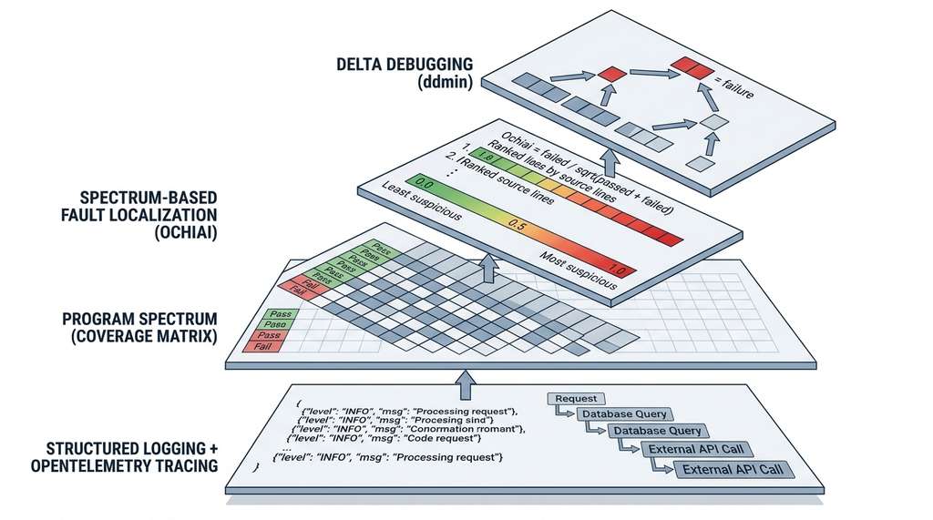
The next section adds an LLM agent layer on top of this infrastructure. The agent reads the ranked suspicious lines, examines the structured log context, formulates root-cause hypotheses, and generates targeted patches. The infrastructure built here provides the agent with precisely the kind of structured, machine-readable evidence it needs to reason effectively about code failures.