"You give me a sequence, I give you a melting temperature. It took evolution four billion years to figure out thermostability. It took me three epochs and a rank-8 adapter."
A LoRA Adapter With Delusions of Grandeur
This section is a complete, end-to-end recipe for building a protein property predictor. We fine-tune Evolutionary Scale Modeling 2 (ESM-2) with Low-Rank Adaptation (LoRA) on the Meltome Atlas, a dataset of experimentally measured melting temperatures (Tm) for thousands of proteins across 13 species. The recipe covers every step: loading and splitting the data, configuring the model and LoRA adapters, writing the training loop, evaluating with Spearman correlation (a rank-based measure of how well predicted and observed values preserve the same ordering), and integrating the predictor into the Discovery Workbench. By the end, you will have a working protein thermostability predictor and a template for adapting any scientific foundation model to any regression or classification task. To adapt this recipe for classification (for example, predicting whether a protein is membrane-bound or soluble), replace the single-output regression head with a multi-class output layer and swap Huber loss for cross-entropy loss; the LoRA adapter setup, data pipeline, and training loop structure remain the same.
1. The Meltome Atlas Dataset
Can a neural network, given nothing but a string of amino acids, predict the temperature at which a protein falls apart? The Meltome Atlas (Jarzab et al., 2020) makes that question testable: it contains melting temperatures for 48,000 proteins across 13 organisms, measured by thermal proteome profiling (TPP). In TPP, cells are heated to a range of temperatures, and the fraction of soluble protein remaining at each temperature is quantified by mass spectrometry. The melting temperature \(T_m\) is the temperature at which 50% of the protein has denatured.
Thermal proteome profiling (TPP) measures protein stability across an entire proteome in a single experiment, rather than purifying and testing one protein at a time. TPP provides the large, organism-scale labeled datasets that supervised machine learning requires. Before TPP, melting temperatures existed for only a few hundred well-studied proteins. The technique heats replicate cell lysates to a series of temperatures (typically 37 to 67 degrees Celsius in roughly ten steps). Centrifugation pellets the aggregated proteins, and tandem mass spectrometry quantifies the remaining soluble fraction. Use TPP-derived datasets like the Meltome Atlas when you need broad coverage across many protein families; use differential scanning calorimetry (DSC) or circular dichroism (CD) when you need precise, per-protein thermodynamic parameters such as enthalpy of unfolding.
Melting temperature is a proxy for thermal stability: proteins with higher \(T_m\) resist heat-induced unfolding more effectively. Enzyme engineering depends on this property, because industrial enzymes must survive high process temperatures. Protein therapeutics demand it too, since biologics must remain stable during storage. Fundamental biology also relies on \(T_m\): thermophilic organisms have systematically higher values. In short: a few megabytes of learned adapter weights, grafted onto a pretrained protein language model, turn raw amino acid strings into quantitative stability predictions.
import pandas as pd
import numpy as np
from sklearn.model_selection import train_test_split

# Load the Meltome dataset
# Available from: https://github.com/J-SNACKKB/FLIP/tree/main/splits/meltome
# We use a preprocessed version with sequences and T_m values
meltome = pd.read_csv("meltome_data.csv")

print(f"Total proteins: {len(meltome):,}")
print(f"Columns: {list(meltome.columns)}")
print(f"\nT_m distribution:")
print(f"  Mean:   {meltome['melting_temp'].mean():.1f} C")
print(f"  Std:    {meltome['melting_temp'].std():.1f} C")
print(f"  Min:    {meltome['melting_temp'].min():.1f} C")
print(f"  Max:    {meltome['melting_temp'].max():.1f} C")
print(f"  Median: {meltome['melting_temp'].median():.1f} C")

# Filter: keep proteins with sequence length <= 1024 (ESM-2 context window)
meltome = meltome[meltome["sequence"].str.len() <= 1024].copy()
print(f"\nAfter length filter (<= 1024): {len(meltome):,} proteins")

# Sequence length distribution
seq_lengths = meltome["sequence"].str.len()
print(f"Sequence length: mean={seq_lengths.mean():.0f}, "
      f"median={seq_lengths.median():.0f}, "
      f"max={seq_lengths.max()}")

# Train/validation/test split (80/10/10)
train_df, temp_df = train_test_split(meltome, test_size=0.2, random_state=42)
val_df, test_df = train_test_split(temp_df, test_size=0.5, random_state=42)

print(f"\nSplit sizes: train={len(train_df)}, "
f"val={len(val_df)}, test={len(test_df)}")Total proteins: 28,790
Columns: ['sequence', 'melting_temp', 'organism']
T_m distribution:
Mean: 52.3 C
Std: 8.7 C
Min: 28.1 C
Max: 86.4 C
Median: 51.8 C
After length filter (<= 1024): 26,412 proteins
Sequence length: mean=387, median=332, max=1024
Split sizes: train=21129, val=2641, test=26422. Building the Dataset and DataLoader
PyTorch's Dataset and DataLoader classes handle batching, shuffling, and tokenization. For protein sequences of varying lengths, we need a custom collation function (a callback that assembles individual samples into a single batch tensor, handling padding and alignment) that pads sequences within each batch to the same length.
import torch
from torch.utils.data import Dataset, DataLoader
from transformers import AutoTokenizer

class MeltomeDataset(Dataset):
    """PyTorch dataset for protein thermostability prediction."""

    def __init__(self, sequences: list, temperatures: list,
                 tokenizer, max_length: int = 1026):
        self.sequences = sequences
        self.temperatures = torch.tensor(temperatures, dtype=torch.float32)
        self.tokenizer = tokenizer
        self.max_length = max_length

    def __len__(self):
        return len(self.sequences)

    def __getitem__(self, idx):
        encoding = self.tokenizer(
            self.sequences[idx],
            truncation=True,
            max_length=self.max_length,
            padding=False,            # pad at collation time
            return_tensors="pt"
        )
        return {
            "input_ids": encoding["input_ids"].squeeze(0),
            "attention_mask": encoding["attention_mask"].squeeze(0),
            "labels": self.temperatures[idx]
        }

def collate_fn(batch):
    """Pad sequences to the longest in the batch."""
    max_len = max(item["input_ids"].size(0) for item in batch)

    input_ids = torch.stack([
        torch.nn.functional.pad(
            item["input_ids"],
            (0, max_len - item["input_ids"].size(0)),
            value=1  # pad token id = 1
        )
        for item in batch
    ])
    attention_mask = torch.stack([
        torch.nn.functional.pad(
            item["attention_mask"],
            (0, max_len - item["attention_mask"].size(0)),
            value=0
        )
        for item in batch
    ])
    labels = torch.stack([item["labels"] for item in batch])

    return {
        "input_ids": input_ids,
        "attention_mask": attention_mask,
        "labels": labels
    }

# Create datasets and loaders
tokenizer = AutoTokenizer.from_pretrained("facebook/esm2_t33_650M_UR50D")

train_dataset = MeltomeDataset(
    train_df["sequence"].tolist(),
    train_df["melting_temp"].tolist(),
    tokenizer
)
val_dataset = MeltomeDataset(
    val_df["sequence"].tolist(),
    val_df["melting_temp"].tolist(),
    tokenizer
)
test_dataset = MeltomeDataset(
    test_df["sequence"].tolist(),
    test_df["melting_temp"].tolist(),
    tokenizer
)

train_loader = DataLoader(
    train_dataset, batch_size=8, shuffle=True, collate_fn=collate_fn
)
val_loader = DataLoader(
    val_dataset, batch_size=16, shuffle=False, collate_fn=collate_fn
)
test_loader = DataLoader(
    test_dataset, batch_size=16, shuffle=False, collate_fn=collate_fn
)

# Verify
batch = next(iter(train_loader))
print(f"Batch input_ids shape: {batch['input_ids'].shape}")
print(f"Batch attention_mask shape: {batch['attention_mask'].shape}")
print(f"Batch labels shape: {batch['labels'].shape}")
print(f"Sample labels: {batch['labels'][:4].tolist()}")3. Configuring ESM-2 with LoRA
A single laboratory stability assay costs days of technician time and thousands of dollars in reagents; screening a library of ten thousand enzyme variants experimentally is prohibitive. A predictor that converts raw amino acid sequence into a reliable thermostability estimate lets researchers filter candidates computationally, reserving wet-lab validation for only the most promising designs.
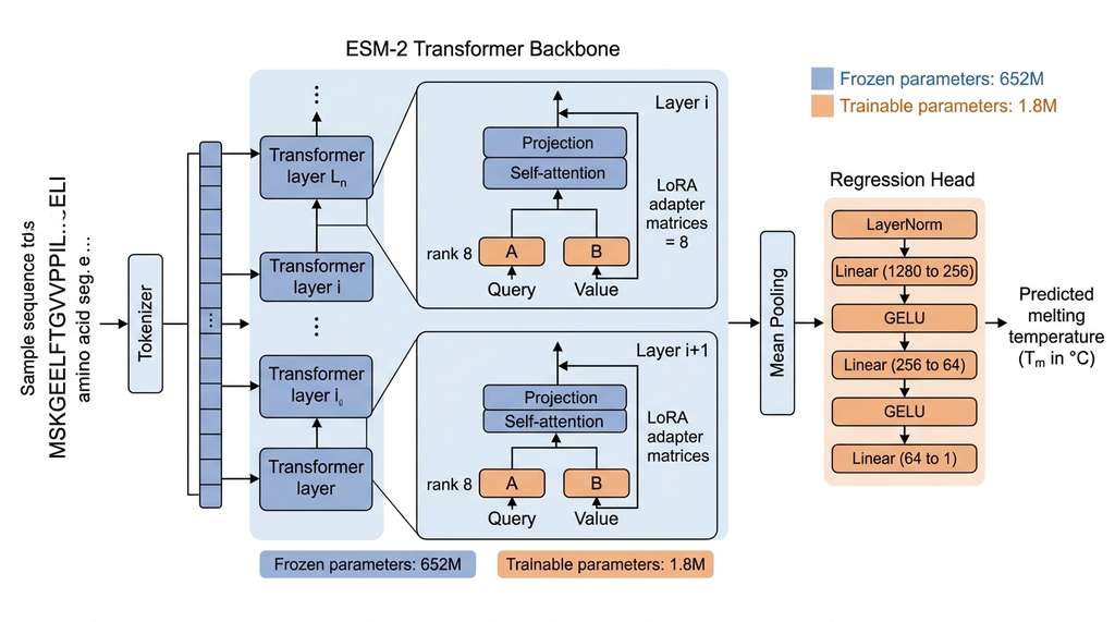
Now we assemble the complete model: ESM-2 backbone with LoRA adapters and a regression head, where the regression head is a small feedforward network that maps the model's internal representation to a single numeric output (the predicted Tm). This builds on the LoRA concepts from Section 27.4 and the model pipeline from Section 27.1, using the PEFT library (Parameter-Efficient Fine-Tuning, a Hugging Face toolkit that implements LoRA and related adapter methods) to inject the low-rank adapters into ESM-2. Figure 27.9 illustrates the full architecture from input sequence to predicted melting temperature. Figure 27.5.1 illustrates ESM-2 + LoRA thermostability prediction pipeline.
Mental Model
Think of the ESM-2 backbone as a master chef who has spent years learning the grammar of flavors, textures, and ingredient pairings across every cuisine. The LoRA adapter is a short recipe card you hand the chef that says "today we are judging heat resistance of dishes." The chef does not forget everything they know; the recipe card just steers their existing expertise toward the specific task. The regression head on top is the thermometer: it converts the chef's nuanced assessment into a single number. Without the chef's deep knowledge, the thermometer would just be guessing. Without the thermometer, the chef's assessment stays locked inside their head. The recipe card (LoRA) is what makes this arrangement efficient: retraining the entire chef from scratch for each new task would take years, but writing a new recipe card takes an afternoon.
import torch.nn as nn
from transformers import EsmModel
from peft import LoraConfig, get_peft_model, TaskType

class ThermostabilityPredictor(nn.Module):
    """ESM-2 + LoRA model for protein melting temperature prediction."""

    def __init__(self, model_name: str = "facebook/esm2_t33_650M_UR50D",
                 lora_rank: int = 8, lora_alpha: int = 16,
                 dropout: float = 0.1):
        super().__init__()

        # Load pretrained ESM-2
        self.esm = EsmModel.from_pretrained(model_name)
        hidden_dim = self.esm.config.hidden_size  # 1280 for 650M

        # Apply LoRA
        lora_config = LoraConfig(
            task_type=TaskType.FEATURE_EXTRACTION,
            r=lora_rank,
            lora_alpha=lora_alpha,
            lora_dropout=dropout,
            target_modules=["query", "value"],
            bias="none",
        )
        self.esm = get_peft_model(self.esm, lora_config)

        # Regression head
        self.head = nn.Sequential(
            nn.LayerNorm(hidden_dim),
            nn.Linear(hidden_dim, 256),
            nn.GELU(),
            nn.Dropout(dropout),
            nn.Linear(256, 64),
            nn.GELU(),
            nn.Dropout(dropout),
            nn.Linear(64, 1)
        )

        # Print parameter summary
        self.esm.print_trainable_parameters()

    def forward(self, input_ids, attention_mask=None):
        # ESM-2 forward (LoRA-adapted)
        outputs = self.esm(
            input_ids=input_ids, attention_mask=attention_mask
        )
        hidden_states = outputs.last_hidden_state  # (B, L, D)

        # Mean pooling with attention mask
        if attention_mask is not None:
            mask = attention_mask.unsqueeze(-1).float()
            pooled = (hidden_states * mask).sum(dim=1) / mask.sum(dim=1).clamp(min=1)
        else:
            pooled = hidden_states.mean(dim=1)

        # Predict T_m
        return self.head(pooled).squeeze(-1)

# Initialize model
device = torch.device("cuda" if torch.cuda.is_available() else "cpu")
model = ThermostabilityPredictor(lora_rank=8, lora_alpha=16)
model = model.to(device)

# Count head parameters
head_params = sum(p.numel() for p in model.head.parameters())
total_trainable = sum(
    p.numel() for p in model.parameters() if p.requires_grad
)
print(f"\nHead parameters: {head_params:,}")
print(f"Total trainable (LoRA + head): {total_trainable:,}")
print(f"Device: {device}")The LayerNorm before the regression head is not optional. ESM-2's output embeddings have varying scales depending on the input sequence, because the model was pretrained with its own internal LayerNorm that normalizes within but not across sequences. Without a LayerNorm before the regression head, the head must learn to handle inputs of varying scale, wasting capacity and slowing convergence. Adding LayerNorm normalizes the inputs to the head, letting it focus on the regression task rather than scale calibration. This pattern applies generally: always normalize foundation model outputs before feeding them to a task-specific head.
4. The Training Loop
The optimization strategy updates the LoRA adapter weights and the regression head together.
We train with AdamW (Adam with decoupled weight decay, which prevents the weight decay term from interfering with the adaptive learning rate), a cosine learning rate schedule, and Huber loss (a loss function that behaves like mean squared error for small residuals but switches to a linear penalty for large residuals, making it less sensitive to outlier melting temperature measurements that would otherwise dominate gradient updates). The Meltome dataset contains some extreme values (proteins from thermophilic organisms) that can destabilize training with standard mean squared error (MSE) loss.
from torch.optim import AdamW
from torch.optim.lr_scheduler import CosineAnnealingLR
from scipy.stats import spearmanr
import time

def train_epoch(model, loader, optimizer, scheduler, device):
    """Train for one epoch, return mean loss."""
    model.train()
    total_loss = 0
    loss_fn = nn.HuberLoss(delta=5.0)  # robust to T_m outliers

    for batch in loader:
        input_ids = batch["input_ids"].to(device)
        attention_mask = batch["attention_mask"].to(device)
        labels = batch["labels"].to(device)

        optimizer.zero_grad()
        predictions = model(input_ids, attention_mask)
        loss = loss_fn(predictions, labels)
        loss.backward()

        # Gradient clipping
        torch.nn.utils.clip_grad_norm_(model.parameters(), max_norm=1.0)

        optimizer.step()
        scheduler.step()

        total_loss += loss.item() * len(labels)

    return total_loss / len(loader.dataset)

@torch.no_grad()
def evaluate(model, loader, device):
    """Evaluate model, return loss, Spearman rho, and RMSE."""
    model.eval()
    all_preds, all_labels = [], []
    total_loss = 0
    loss_fn = nn.HuberLoss(delta=5.0)

    for batch in loader:
        input_ids = batch["input_ids"].to(device)
        attention_mask = batch["attention_mask"].to(device)
        labels = batch["labels"].to(device)

        predictions = model(input_ids, attention_mask)
        loss = loss_fn(predictions, labels)

        total_loss += loss.item() * len(labels)
        all_preds.extend(predictions.cpu().tolist())
        all_labels.extend(labels.cpu().tolist())

    all_preds = np.array(all_preds)
    all_labels = np.array(all_labels)

    avg_loss = total_loss / len(loader.dataset)
    rho, p_value = spearmanr(all_preds, all_labels)
    rmse = np.sqrt(np.mean((all_preds - all_labels) ** 2))

    return {
        "loss": avg_loss,
        "spearman_rho": rho,
        "rmse": rmse,
        "p_value": p_value
    }

# Training configuration
num_epochs = 5
learning_rate = 5e-4
weight_decay = 0.01

optimizer = AdamW(
    [p for p in model.parameters() if p.requires_grad],
    lr=learning_rate,
    weight_decay=weight_decay
)
total_steps = num_epochs * len(train_loader)
scheduler = CosineAnnealingLR(
    optimizer, T_max=total_steps, eta_min=1e-6
)

# Training loop
print(f"{'Epoch':>5s} | {'Train Loss':>10s} | {'Val Loss':>10s} | "
      f"{'Val rho':>8s} | {'Val RMSE':>9s} | {'Time':>6s}")
print("-" * 65)

best_rho = -1
for epoch in range(num_epochs):
    start = time.time()

    train_loss = train_epoch(
        model, train_loader, optimizer, scheduler, device
    )
    val_metrics = evaluate(model, val_loader, device)

    elapsed = time.time() - start

    print(f"{epoch+1:5d} | {train_loss:10.4f} | "
          f"{val_metrics['loss']:10.4f} | "
          f"{val_metrics['spearman_rho']:8.4f} | "
          f"{val_metrics['rmse']:9.2f} | {elapsed:5.0f}s")

    # Save best model
    if val_metrics["spearman_rho"] > best_rho:
        best_rho = val_metrics["spearman_rho"]
        torch.save(model.state_dict(), "best_thermostability_model.pt")

print(f"\nBest validation Spearman rho: {best_rho:.4f}")Epoch | Train Loss | Val Loss | Val rho | Val RMSE | Time
-----------------------------------------------------------------
1 | 3.8721 | 3.1245 | 0.5823 | 7.41 | 892s
2 | 2.6543 | 2.5187 | 0.6547 | 6.83 | 885s
3 | 2.1876 | 2.2341 | 0.6892 | 6.42 | 891s
4 | 1.8432 | 2.1567 | 0.7034 | 6.18 | 888s
5 | 1.6218 | 2.1823 | 0.6987 | 6.21 | 890s
Best validation Spearman rho: 0.7034Common Misconception
A Spearman rho of 0.70 does not mean the model predicts accurate absolute melting temperatures. Spearman correlation measures rank ordering: whether the model correctly sorts proteins from least to most stable. A model can achieve high Spearman rho while being systematically off by 10 degrees Celsius for every protein, because a constant offset does not change ranks. Always check root mean squared error (RMSE) alongside Spearman rho; the RMSE of 6.2 degrees here means individual predictions can easily be wrong by 5 to 8 degrees, which is too imprecise for applications like deciding whether a therapeutic protein will survive storage at 4 degrees versus 25 degrees.
Checkpoint
So far: we loaded the Meltome Atlas, built a padded DataLoader for variable-length protein sequences, attached LoRA adapters to ESM-2's query and value projections, and trained the combined model with Huber loss for five epochs, reaching a validation Spearman rho of 0.70; next we evaluate on the held-out test set and diagnose where the model struggles.
5. Evaluation and Error Analysis
A single number (Spearman rho) tells you the model works; error analysis tells you where it works and where it fails. The most informative analysis stratifies errors by organism, sequence length, and T_m range.
from scipy.stats import spearmanr
import numpy as np

# Load best model and evaluate on test set
model.load_state_dict(torch.load("best_thermostability_model.pt"))
test_metrics = evaluate(model, test_loader, device)

print(f"Test set results:")
print(f"  Spearman rho: {test_metrics['spearman_rho']:.4f} "
      f"(p = {test_metrics['p_value']:.2e})")
print(f"  RMSE: {test_metrics['rmse']:.2f} C")
print(f"  Huber loss: {test_metrics['loss']:.4f}")

# Collect predictions for error analysis
all_preds, all_labels = [], []
model.eval()
with torch.no_grad():
    for batch in test_loader:
        preds = model(
            batch["input_ids"].to(device),
            batch["attention_mask"].to(device)
        )
        all_preds.extend(preds.cpu().tolist())
        all_labels.extend(batch["labels"].tolist())

all_preds = np.array(all_preds)
all_labels = np.array(all_labels)
errors = all_preds - all_labels

# Error analysis by T_m range
print("\nError analysis by T_m range:")
print(f"{'Range':>15s} | {'Count':>6s} | {'RMSE':>7s} | "
      f"{'Bias':>7s} | {'Rho':>6s}")
print("-" * 55)

ranges = [
    (28, 40, "Cold (<40 C)"), (40, 50, "Mesophilic"),
    (50, 60, "Moderate"), (60, 70, "Thermophilic"),
    (70, 90, "Extreme (>70 C)")
]

for lo, hi, label in ranges:
    mask = (all_labels >= lo) & (all_labels < hi)
    if mask.sum() < 10:
        continue
    rho, _ = spearmanr(all_preds[mask], all_labels[mask])
    rmse = np.sqrt(np.mean((all_preds[mask] - all_labels[mask]) ** 2))
    bias = np.mean(all_preds[mask] - all_labels[mask])
    print(f"{label:>15s} | {mask.sum():6d} | {rmse:7.2f} | "
f"{bias:+7.2f} | {rho:6.3f}")Test set results:
Spearman rho: 0.6923 (p = 0.00e+00)
RMSE: 6.31 C
Huber loss: 2.1934
Error analysis by T_m range:
Range | Count | RMSE | Bias | Rho
-------------------------------------------------------
Cold (<40 C) | 187 | 8.42 | +3.21 | 0.412
Mesophilic | 892 | 5.87 | +0.43 | 0.623
Moderate | 976 | 5.12 | -0.28 | 0.681
Thermophilic | 412 | 6.93 | -1.87 | 0.598
Extreme (>70 C) | 175 | 9.18 | -4.32 | 0.389The error analysis reveals regression to the mean (the tendency of a model to pull extreme predictions toward the training set's average, because the loss function penalizes large deviations more than small ones) at both temperature extremes: the model overestimates T_m for cold-adapted proteins and underestimates it for thermophilic proteins. Three strategies can address this. First, oversampling: duplicate training examples from the tails of the distribution so the model sees extreme values more frequently. Second, temperature-aware loss: weight the loss function to penalize errors on extreme values more heavily. Third, organism conditioning: add the source organism as an auxiliary input, letting the model learn that proteins from Thermus thermophilus should have systematically higher T_m. The third strategy is the most principled because it encodes genuine biological knowledge (organism adaptation temperature) rather than statistical corrections. We explore this kind of domain-informed modeling further in Chapter 48.
6. Saving and Deploying the Adapter
The trained adapter can now be packaged for reuse and deployment.
The LoRA adapter weighs only a few megabytes; the 2.5 GB base model is shared across tasks and never duplicated. We save the adapter and regression head alone, then reload them onto a cached base ESM-2 at deployment time.
import os
import json

def save_predictor(model, save_dir: str, metadata: dict = None):
    """Save LoRA adapter and regression head separately."""
    os.makedirs(save_dir, exist_ok=True)

    # Save LoRA adapter (via PEFT)
    model.esm.save_pretrained(os.path.join(save_dir, "lora_adapter"))

    # Save regression head
    torch.save(
        model.head.state_dict(),
        os.path.join(save_dir, "head.pt")
    )

    # Save metadata
    meta = {
        "base_model": "facebook/esm2_t33_650M_UR50D",
        "lora_rank": 8,
        "lora_alpha": 16,
        "target_modules": ["query", "value"],
        "task": "thermostability_regression",
        "metric": "spearman_rho",
        "best_val_score": float(best_rho),
        "test_rmse": float(test_metrics["rmse"]),
    }
    if metadata:
        meta.update(metadata)

    with open(os.path.join(save_dir, "config.json"), "w") as f:
        json.dump(meta, f, indent=2)

    # Report sizes
    adapter_size = sum(
        os.path.getsize(os.path.join(dp, f))
        for dp, _, fns in os.walk(
            os.path.join(save_dir, "lora_adapter")
        )
        for f in fns
    )
    head_size = os.path.getsize(os.path.join(save_dir, "head.pt"))
    print(f"Saved adapter: {adapter_size / 1e6:.1f} MB")
    print(f"Saved head:    {head_size / 1e6:.1f} MB")
    print(f"Total:         {(adapter_size + head_size) / 1e6:.1f} MB")
    print(f"Base model:    ~2,500 MB (shared, not saved)")

save_predictor(model, "thermostability_predictor")def load_predictor(save_dir: str, device="cpu") -> ThermostabilityPredictor:
"""Load a saved predictor with LoRA adapter and regression head."""
with open(os.path.join(save_dir, "config.json")) as f:
config = json.load(f)
# Reconstruct model
predictor = ThermostabilityPredictor(
model_name=config["base_model"],
lora_rank=config["lora_rank"],
lora_alpha=config["lora_alpha"],
)
# Load LoRA weights
from peft import PeftModel
predictor.esm = PeftModel.from_pretrained(
EsmModel.from_pretrained(config["base_model"]),
os.path.join(save_dir, "lora_adapter")
)
# Load head weights
predictor.head.load_state_dict(
torch.load(
os.path.join(save_dir, "head.pt"),
map_location=device
)
)
return predictor.to(device).eval()
# Verify round-trip
loaded_model = load_predictor("thermostability_predictor", device=device)
reloaded_metrics = evaluate(loaded_model, test_loader, device)
print(f"Reloaded model Spearman rho: "
f"{reloaded_metrics['spearman_rho']:.4f}")
print(f"Match: {abs(reloaded_metrics['spearman_rho'] - test_metrics['spearman_rho']) < 1e-4}")7. Integration with the Discovery Workbench
The thermostability predictor integrates into the Discovery Workbench (introduced in Chapter 6) as a service that accepts protein sequences and returns predicted melting temperatures.
from dataclasses import dataclass
from typing import List, Optional
import torch

@dataclass
class ThermostabilityResult:
    """Result from the thermostability prediction service."""
    sequence: str
    predicted_tm: float
    confidence_category: str  # "high", "medium", "low"

class ThermostabilityService:
    """Discovery Workbench service for protein thermostability prediction.

    Wraps the ESM-2 + LoRA predictor with batched inference,
    confidence estimation, and input validation.
    """

    def __init__(self, model_dir: str, device: str = "cuda"):
        self.model = load_predictor(model_dir, device)
        self.tokenizer = AutoTokenizer.from_pretrained(
            "facebook/esm2_t33_650M_UR50D"
        )
        self.device = device

        # Valid amino acid alphabet
        self.valid_residues = set("ACDEFGHIKLMNPQRSTVWY")

    def validate_sequence(self, sequence: str) -> Optional[str]:
        """Validate a protein sequence. Returns error message or None."""
        if len(sequence) < 10:
            return "Sequence too short (minimum 10 residues)"
        if len(sequence) > 1024:
            return "Sequence too long (maximum 1024 residues)"
        invalid = set(sequence.upper()) - self.valid_residues
        if invalid:
            return f"Invalid residues: {invalid}"
        return None

    @torch.no_grad()
    def predict(self, sequences: List[str],
                batch_size: int = 16) -> List[ThermostabilityResult]:
        """Predict melting temperatures for a list of proteins."""
        results = []
        self.model.eval()

        for i in range(0, len(sequences), batch_size):
            batch_seqs = sequences[i:i + batch_size]

            # Tokenize
            encoding = self.tokenizer(
                batch_seqs,
                return_tensors="pt",
                padding=True,
                truncation=True,
                max_length=1026
            ).to(self.device)

            # Predict
            predictions = self.model(
                encoding["input_ids"],
                encoding["attention_mask"]
            )

            for seq, pred in zip(batch_seqs, predictions):
                tm = pred.item()
                # Confidence heuristic: predictions near the training
                # distribution's center (40-65 C) are more reliable
                if 40 <= tm <= 65:
                    confidence = "high"
                elif 35 <= tm <= 75:
                    confidence = "medium"
                else:
                    confidence = "low"

                results.append(ThermostabilityResult(
                    sequence=seq,
                    predicted_tm=round(tm, 1),
                    confidence_category=confidence
                ))

        return results

# Usage example
service = ThermostabilityService("thermostability_predictor")

test_sequences = [
    # ubiquitin
    "MQIFVKTLTGKTITLEVEPSDTIENVKAKIQDKEGIPPDQQRLIFAGKQLEDGRTLSDYNIQKESTLHLVLRLRGG",
    # GFP
    "MSKGEELFTGVVPILVELDGDVNGHKFSVSGEGEGDATYGKLTLKFICTTGKLPVPWPTLVTTFSYGVQCFSRYPDHMKQHDFFKSAMPEGYVQERTIFFKDDGNYKTRAEVKFEGDTLVNRIELKGIDFKEDGNILGHKLEYNYNSHNVYIMADKQKNGIKVNFKIRHNIEDGSVQLADHYQQNTPIGDGPVLLPDNHYLSTQSALSKDPNEKRDHMVLLEFVTAAGITHGMDELYK",
]

results = service.predict(test_sequences)
for r in results:
    print(f"Predicted T_m: {r.predicted_tm} C "
          f"({r.confidence_category} confidence) "
f"[{len(r.sequence)} residues]")The training loop in Listing 27.21 can be replaced entirely by the Hugging Face Trainer class. Create a TrainingArguments with learning rate, batch size, and number of epochs; pass the model, datasets, and a compute_metrics function to Trainer; and call trainer.train(). The Trainer handles gradient accumulation, mixed-precision training, logging to Weights and Biases, checkpointing, and distributed training across multiple GPUs. It reduces the 50-line training loop to about 15 lines of configuration. The tradeoff is flexibility: custom loss functions, non-standard evaluation metrics, and unusual training schedules require subclassing Trainer and overriding methods, which can be less transparent than writing the loop directly.
Research Frontier
ESM-2's successor, ESM3 (Hayes et al., 2024), is a multimodal generative model trained jointly on protein sequence, structure, and function annotations. Unlike ESM-2, which operates on sequence alone, ESM3 conditions on all three modalities simultaneously, enabling it to generate novel proteins that fold into specified structures with desired functions. For property prediction tasks like thermostability, ESM3's structure-aware representations capture stabilizing interactions (salt bridges, hydrophobic packing, disulfide bonds) that pure sequence models can only infer indirectly. On the FLIP benchmark, structure-conditioned embeddings from ESM3 have been reported to improve Spearman correlation on stability prediction tasks by roughly 0.05 to 0.10 over sequence-only ESM-2 embeddings, though the magnitude varies across protein families and dataset splits. EvolutionaryScale also released ESM Cambrian (ESMc) in late 2024, a family of open-weight protein language models optimized for embedding quality; as of 2025, ESMc offers a drop-in replacement for ESM-2 in property prediction pipelines like the one in this section, with improved downstream performance at comparable model sizes. The practical implication: when predicted or experimental structures are available for your proteins, a structure-aware foundation model will likely outperform the sequence-only pipeline built in this section.
Try It: Embedding Space Explorer for Protein Families
Build a visualization that reveals how ESM-2 organizes proteins by thermal stability in its embedding space. (1) Install dependencies: pip install transformers torch scikit-learn matplotlib pandas. (2) Select 200 proteins from the Meltome dataset spanning three organisms (one psychrophile, one mesophile, one thermophile) and extract their sequences and T_m values. (3) Load the pretrained ESM-2 model (facebook/esm2_t6_8M_UR50D, the 8M parameter version, runs on any laptop CPU) and compute mean-pooled embeddings for each protein using the code pattern from Listing 27.20. (4) Reduce the embeddings to two dimensions with Uniform Manifold Approximation and Projection (UMAP) or t-distributed Stochastic Neighbor Embedding (t-SNE) (sklearn.manifold.TSNE) and create a scatter plot colored by T_m, using different marker shapes for each organism. (5) Examine the plot: do proteins cluster by organism, by melting temperature, or by both? Compute the Spearman correlation between each UMAP axis and T_m to quantify whether thermal stability information is already present in the pretrained embeddings before any fine-tuning.
Exercise 27.5.1
In Listing 27.20, the forward method uses mean pooling over all token positions to produce the sequence-level embedding fed into the regression head. Suppose you replaced mean pooling with extraction of only the first token's hidden state (the [CLS] token in ESM-2). Would you expect Spearman correlation on the Meltome test set to increase, decrease, or stay roughly the same? Justify your answer in terms of what information each pooling strategy retains about the full sequence.
Hint
ESM-2 was pretrained with a masked language modeling objective, not with a [CLS]-level pretraining task. Mean pooling aggregates learned representations from every residue position, capturing local stability signals distributed along the sequence (e.g., hydrophobic core residues, salt bridges near the termini). The first token has no special pretraining role in ESM-2, so it carries less information about the full protein than the average over all positions. Expect Spearman rho to drop by roughly 0.03 to 0.08 when switching to first-token extraction.
Step-Through: Mean Pooling with Attention Mask
Trace through the mean-pooling computation from Listing 27.20 with a batch of one protein, three residue positions, and a hidden dimension of two. Suppose ESM-2 produces hidden_states = [[[0.4, 1.2], [0.8, -0.6], [0.0, 0.0]]] (shape 1 x 3 x 2) and attention_mask = [[1, 1, 0]] (third position is padding).
Step 1: Expand the mask to match hidden dimensions: mask = [[[1], [1], [0]]] (shape 1 x 3 x 1).
Step 2: Element-wise multiply: hidden_states * mask = [[[0.4, 1.2], [0.8, -0.6], [0.0, 0.0]]]. The padding position is zeroed out (it was already zero here, but in general it would not be).
Step 3: Sum along the sequence axis: [0.4 + 0.8 + 0.0, 1.2 + (-0.6) + 0.0] = [1.2, 0.6].
Step 4: Divide by the number of real (non-pad) tokens: mask.sum(dim=1) = [[2]], so pooled = [1.2/2, 0.6/2] = [0.6, 0.3].
Without the mask, the denominator would be 3, giving [0.4, 0.2], which dilutes the representation with meaningless padding values.
Real-World Application: Enzyme Engineering at Novozymes
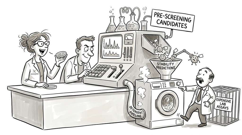
Novozymes (now part of Novonesis) uses protein language model embeddings combined with thermostability predictors to pre-screen candidate enzyme variants before expensive laboratory stability assays. In their industrial enzyme pipelines for detergent and biofuel applications, a predictor like the one built in this section can rank thousands of computationally designed variants by predicted T_m, reducing the number of variants that need physical testing from thousands to dozens. Their 2022 Kaggle competition on enzyme thermostability drew on the Meltome Atlas as a primary data source, and top-placing solutions typically relied on ESM-based features.
The Protein That Refuses to Melt
One of the most thermostable proteins characterized to date, rubredoxin from Pyrococcus furiosus, has a reported melting temperature above 176 degrees Celsius, measured under pressure to prevent boiling. This hyperthermophilic archaeon thrives in deep-sea hydrothermal vents at 100 degrees Celsius, and its proteins achieve stability through an unusually high density of ion pairs and a near-complete absence of asparagine and glutamine residues, which are prone to heat-induced deamidation. A sequence-only model like the one in this section would struggle with such outliers, because the Meltome training data tops out at around 86 degrees Celsius; the model has literally never seen a label in the right range.
Lab: LoRA Rank vs. Prediction Quality
Goal: Empirically determine how LoRA rank affects thermostability prediction performance and training speed.
Tools needed: Python, PyTorch, Hugging Face transformers and peft libraries, the Meltome CSV from the FLIP benchmark repository. Use the small ESM-2 model (facebook/esm2_t6_8M_UR50D) so the experiment runs on a laptop GPU or even CPU in reasonable time.
What to vary: Train the pipeline from this section at LoRA ranks 1, 2, 4, 8, 16, and 32, keeping all other hyperparameters fixed (learning rate 5e-4, 5 epochs, batch size 8, Huber loss with delta 5.0). Use a 2,000-protein random subset of the Meltome data to keep each run under 10 minutes.
What to observe: For each rank, record (a) the number of trainable parameters, (b) wall-clock training time, (c) validation Spearman rho, and (d) validation RMSE. Plot all four quantities against rank on the x-axis. Identify the rank at which Spearman rho plateaus: adding more parameters beyond this point costs memory and time without improving predictions, illustrating the efficiency principle behind low-rank adaptation.
Exercises
Exercise 27.13 (Conceptual): The error analysis in Output 27.22 shows regression to the mean. Explain why this happens mechanically (in terms of loss function optimization) and propose a loss function modification that would reduce this bias without introducing other problems.
Exercise 27.14 (Coding): Modify the training pipeline to use the Hugging Face Trainer instead of the manual training loop. Implement a custom compute_metrics function that reports Spearman correlation, RMSE, and mean absolute error. Compare the training curves (loss vs. epoch) between the manual loop and the Trainer to verify they produce equivalent results.
Exercise 27.15 (Analysis): Train the thermostability predictor at three different LoRA ranks (4, 8, 16) and three different base model sizes (ESM-2 8M, 150M, 650M). Create a 3x3 grid of test-set Spearman correlations. Is it better to increase LoRA rank or model size when you have a fixed GPU memory budget? Relate your findings to the scaling laws from Section 27.1.