29.1 Chain-of-Thought and Test-Time Compute

"I was asked to solve a differential equation. I could have answered in one token, but instead I wrote a 2,000-token internal monologue. My therapist says this is progress."

A Chain-of-Thought That Became a Chain-of-Consciousness

1. The Chain-of-Thought Revolution

When a language model answers a complex scientific question in a single pass, it often produces a confident number that is quietly, catastrophically wrong. A single misapplied formula or a skipped unit conversion can invalidate an entire analysis, and the model gives no trace of where the error entered. The technique that changed this failure mode arrived in 2022.

What happens when you ask a language model to show its work before answering? In 2022, Wei et al. found out: accuracy on arithmetic, commonsense, and symbolic reasoning tasks jumped by 20 to 60 percentage points. The technique, called chain-of-thought (CoT) prompting, works by forcing the model to decompose a complex problem into smaller subproblems that each fall within its reliable capability range.

Chain-of-thought prompting instructs a large language model to produce explicit intermediate reasoning steps (equations, sub-conclusions, checks) before stating its final answer. It matters because LLMs are autoregressive, where autoregressive means each token is generated one at a time, conditioned on all tokens produced so far. Without written intermediate steps, the model must compress multi-step logic into a single forward pass, which frequently fails on problems requiring more than two reasoning hops. The core mechanism is straightforward: each reasoning step the model writes becomes part of the input context for the next step. This gives the model an external scratchpad that extends its working memory beyond the fixed depth of the transformer. Use CoT whenever a task involves multi-step logic, arithmetic, or causal chains; for single-lookup factual recall or classification tasks with well-separated categories, standard prompting is faster and equally accurate.

The mechanism is straightforward. Consider a graduate-level chemistry question: "What is the pH of a 0.05 M solution of acetic acid (\(K_a = 1.8 \times 10^{-5}\))?" Without CoT, the model must produce the answer in a single forward pass. With CoT, the model can write out the equilibrium expression, set up the Initial, Change, Equilibrium (ICE) table, solve the quadratic approximation, and compute the logarithm as separate, verifiable steps.

Each output token in a transformer is a function of all preceding tokens. When the model writes intermediate steps, those steps enter the context for subsequent computations, expanding "working memory" with every reasoning step. The model uses its own output as a scratchpad, a form of computation augmentation that connects to the Turing machine's tape and the external memory concepts in Section 4.2.

Few-Shot CoT versus Zero-Shot CoT

CoT prompting comes in two flavors. Few-shot CoT provides explicit examples of step-by-step reasoning in the prompt. Zero-shot CoT appends an instruction like "Think step by step" without examples. Few-shot CoT is more reliable for specialized domains (because the examples anchor the reasoning style), but zero-shot CoT is more practical when constructing domain-specific examples is expensive.

For scientific applications, few-shot CoT with domain-specific exemplars typically outperforms zero-shot prompting in published benchmarks. The key is to choose exemplars that demonstrate the reasoning patterns relevant to the target domain, not just the surface format. A chemistry CoT exemplar should demonstrate equilibrium reasoning; a genomics exemplar should demonstrate sequence-to-function inference. In short: letting the model write before it answers turns a lossy single guess into a auditable, correctable chain of smaller guesses.

import anthropic

client = anthropic.Anthropic()

# Few-shot CoT for scientific reasoning
SYSTEM_PROMPT = """You are a scientific reasoning assistant. For every problem:
1. Identify the relevant physical/chemical/mathematical principles
2. Write the governing equations
3. Substitute known values
4. Solve step by step, showing units
5. Verify the answer by checking units and order of magnitude"""

FEW_SHOT_EXEMPLAR = """
Example problem: What is the de Broglie wavelength of an electron
accelerated through 100 V?

Step 1: The de Broglie relation is lambda = h / p, where p is momentum.
Step 2: Kinetic energy equals charge times voltage: KE = eV = (1/2)mv^2.
Step 3: Momentum p = sqrt(2m * KE) = sqrt(2 * m_e * eV).
  m_e = 9.109e-31 kg, e = 1.602e-19 C, V = 100 V
  p = sqrt(2 * 9.109e-31 * 1.602e-19 * 100) = 5.40e-24 kg*m/s
Step 4: lambda = h / p = 6.626e-34 / 5.40e-24 = 1.23e-10 m = 0.123 nm
Step 5: Verification: this is on the order of atomic spacing, which is
physically reasonable for 100 eV electrons.

Answer: 0.123 nm
"""

def scientific_cot(problem: str) -> str:
    """Solve a scientific problem using few-shot chain-of-thought."""
    response = client.messages.create(
        model="claude-sonnet-4-20250514",
        max_tokens=2048,
        system=SYSTEM_PROMPT,
        messages=[
            {"role": "user", "content": FEW_SHOT_EXEMPLAR + "\n\n" + problem}
        ]
    )
    return response.content[0].text

# Solve a new problem using the demonstrated reasoning pattern
result = scientific_cot(
    "What is the pH of a 0.05 M solution of acetic acid (Ka = 1.8e-5)?"
)
print(result)

2. Self-Consistency: Voting Over Reasoning Paths

A single chain of thought can go wrong at any step. Wang et al. (2022, published at ICLR 2023) introduced self-consistency decoding: sample multiple independent reasoning chains for the same problem, extract the final answer from each, and return the answer that appears most frequently. The intuition is that correct reasoning paths are more likely to converge on the same answer, while errors are idiosyncratic and scatter across different wrong answers.

Formally, given a problem \(x\), we sample \(N\) reasoning chains \(\{r_1, \ldots, r_N\}\) at temperature \(T > 0\) (a parameter controlling the randomness of token selection, where higher values produce more diverse outputs), extract answers \(\{a_1, \ldots, a_N\}\), and return:

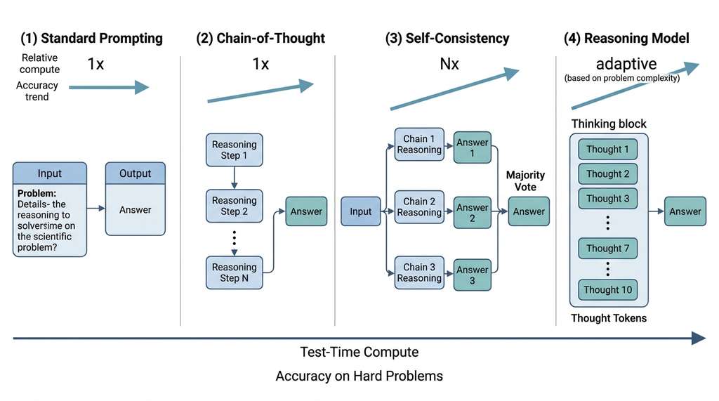
This majority-vote approach requires no additional training. It works because the sampling temperature introduces diversity in reasoning paths while the mathematical structure of the problem constrains correct answers to cluster. Figure 1 illustrates how self-consistency compares to standard and CoT prompting in terms of the inference pipeline. For scientific problems, where numerical answers must be extracted and compared, we typically use approximate equality with a tolerance:

import re
from collections import Counter

def extract_numerical_answer(text: str) -> float | None:
    """Extract the last numerical value from a reasoning trace."""
    # Match numbers in scientific notation or decimal form
    pattern = r'[-+]?\d*\.?\d+(?:[eE][-+]?\d+)?'
    matches = re.findall(pattern, text)
    if matches:
        return float(matches[-1])
    return None

def self_consistency(
    client: anthropic.Anthropic,
    problem: str,
    n_samples: int = 8,
    temperature: float = 0.7,
    tolerance: float = 0.05
) -> dict:
    """Self-consistency decoding: sample multiple CoT paths, majority vote.

    Args:
        client: Anthropic API client
        problem: The problem to solve
        n_samples: Number of independent reasoning chains to sample
        temperature: Sampling temperature (higher = more diverse paths)
        tolerance: Relative tolerance for grouping numerical answers

    Returns:
        Dict with best_answer, confidence, and all sampled chains
    """
    chains = []
    answers = []

    for _ in range(n_samples):
        response = client.messages.create(
            model="claude-sonnet-4-20250514",
            max_tokens=2048,
            temperature=temperature,
            messages=[{
                "role": "user",
                "content": f"Solve step by step:\n{problem}\n\n"
                           f"Show all work, then state the final answer."
            }]
        )
        text = response.content[0].text
        chains.append(text)

        answer = extract_numerical_answer(text)
        if answer is not None:
            answers.append(answer)

    if not answers:
        return {"best_answer": None, "confidence": 0.0, "chains": chains}

    # Group answers by approximate equality
    groups: list[list[float]] = []
    for ans in answers:
        placed = False
        for group in groups:
            if abs(ans - group[0]) / max(abs(group[0]), 1e-10) < tolerance:
                group.append(ans)
                placed = True
                break
        if not placed:
            groups.append([ans])

    # Find the largest group
    best_group = max(groups, key=len)
    confidence = len(best_group) / len(answers)
    best_answer = sum(best_group) / len(best_group)  # average within group

    return {
        "best_answer": best_answer,
        "confidence": confidence,
        "n_agreeing": len(best_group),
        "n_total": len(answers),
        "chains": chains
    }

# Example usage
result = self_consistency(
    client,
    "A projectile is launched at 45 degrees with initial speed 20 m/s. "
    "Ignoring air resistance, what is the maximum height in meters?",
    n_samples=8
)
print(f"Answer: {result['best_answer']:.2f} m")
print(f"Confidence: {result['confidence']:.0%} ({result['n_agreeing']}/{result['n_total']} agree)")

3. The Test-Time Compute Paradigm

The techniques above (CoT prompting and self-consistency) require the user to design the reasoning strategy and control the sampling; the model itself has no notion that it should think longer on harder problems. The next leap built test-time computation directly into the model's architecture and training, removing that burden from the user. This is the approach taken by OpenAI's o1 and o3 models, Anthropic's extended thinking, DeepSeek-R1 (an open-weights reasoning model released in early 2025 that demonstrated competitive performance with proprietary systems), and Google's Gemini Deep Think.

These reasoning models are trained with reinforcement learning to produce long internal reasoning traces before generating a final answer. The model learns to allocate more "thinking tokens" to harder problems. Unlike standard CoT prompting (where the user asks the model to think step by step), reasoning models do this automatically: they have been trained to recognize when a problem requires extended deliberation.

To see why this approach succeeds, consider what happens computationally when the model generates each additional reasoning token.

The key architectural insight is that reasoning tokens provide adaptive computation (the ability to vary how much computation the model spends on each input based on its difficulty). A standard transformer uses a fixed number of layers (fixed computation depth) regardless of problem difficulty. A reasoning model deepens its computation by generating more intermediate tokens, each of which flows through the full transformer stack (where the transformer stack is the sequence of attention and feed-forward layers that every token passes through during a single forward pass). A problem that requires \(k\) reasoning steps gets roughly \(k \times L\) layers of effective depth, where \(L\) is the transformer's layer count.

Using OpenAI's Reasoning Models

The o1 and o3 model families expose reasoning through a "reasoning effort" parameter that controls how many internal tokens the model allocates. Higher effort means more thinking, higher cost, and (on hard problems) higher accuracy. For scientific applications, the tradeoff is explicit: easy calculations need low effort; novel derivations need high effort.

from openai import OpenAI

openai_client = OpenAI()

def reasoning_model_solve(
    problem: str,
    effort: str = "medium"  # "low", "medium", or "high"
) -> dict:
    """Solve a problem using OpenAI's o3 reasoning model.

    The reasoning_effort parameter controls internal compute allocation:
    - "low": fast, suitable for straightforward calculations
    - "medium": balanced, suitable for multi-step derivations
    - "high": thorough, suitable for novel or ambiguous problems
    """
    response = openai_client.chat.completions.create(
        model="o3",
        reasoning_effort=effort,
        messages=[{
            "role": "user",
            "content": problem
        }]
    )

    return {
        "answer": response.choices[0].message.content,
        "reasoning_tokens": response.usage.completion_tokens_details.reasoning_tokens,
        "output_tokens": response.usage.completion_tokens,
        "model": response.model
    }

# Compare effort levels on a graduate-level physics problem
problem = """
A uniform solid sphere of mass M and radius R rolls without slipping
down an inclined plane of angle theta. Derive the acceleration of the
center of mass, showing all steps including the moment of inertia
calculation and the no-slip constraint.
"""

for effort in ["low", "medium", "high"]:
    result = reasoning_model_solve(problem, effort=effort)
    print(f"\nEffort: {effort}")
    print(f"Reasoning tokens: {result['reasoning_tokens']}")
    print(f"Answer preview: {result['answer'][:200]}...")

Using Anthropic's Extended Thinking

Anthropic's Claude models support extended thinking, which exposes the model's internal reasoning process through a dedicated thinking block. Unlike the opaque reasoning tokens in o1/o3, extended thinking returns the full reasoning trace, letting you inspect, debug, and verify each step.

import anthropic

client = anthropic.Anthropic()

def extended_thinking_solve(
    problem: str,
    budget_tokens: int = 10000
) -> dict:
    """Solve a problem using Claude's extended thinking.

    Args:
        problem: The scientific problem to solve
        budget_tokens: Maximum tokens for internal reasoning

    Returns:
        Dict with thinking trace, final answer, and token usage
    """
    response = client.messages.create(
        model="claude-sonnet-4-20250514",
        max_tokens=16000,
        thinking={
            "type": "enabled",
            "budget_tokens": budget_tokens
        },
        messages=[{
            "role": "user",
            "content": problem
        }]
    )

    thinking_text = ""
    answer_text = ""
    for block in response.content:
        if block.type == "thinking":
            thinking_text = block.thinking
        elif block.type == "text":
            answer_text = block.text

    return {
        "thinking": thinking_text,
        "answer": answer_text,
        "input_tokens": response.usage.input_tokens,
        "output_tokens": response.usage.output_tokens
    }

# Solve a problem that requires extended reasoning
result = extended_thinking_solve(
    "Prove that the sum of the first n odd numbers equals n^2. "
    "Use mathematical induction and show every step.",
    budget_tokens=8000
)

print("=== THINKING TRACE ===")
print(result["thinking"][:1000])
print("\n=== FINAL ANSWER ===")
print(result["answer"][:500])

4. When Reasoning Models Fail

Reasoning models are not infallible. They exhibit systematic failure modes that practitioners must recognize:

Hallucinated reasoning steps. A model may produce a chain of thought that looks correct on the surface but contains a subtle mathematical error in step 3 of 7. The remaining steps are internally consistent given the wrong intermediate result, making the error hard to detect by inspection. This is why process reward models (Section 29.2) evaluate each step independently.

Reasoning anchoring. Once a model commits to an approach in its early reasoning tokens, it rarely backtracks. If the initial approach is wrong, the model will often force-fit the remaining steps rather than reconsidering. This is analogous to the anchoring bias (a cognitive bias in which an initial piece of information disproportionately influences subsequent judgments) in human cognition and is a fundamental limitation of autoregressive generation: tokens flow left to right, and the model cannot "undo" earlier reasoning.

Structural and Distributional Limits

Distribution shift. Reasoning models are trained on problems (and reasoning traces) drawn from their training distribution. When presented with a genuinely novel problem type, the model may apply familiar-looking but inappropriate reasoning templates. For scientific discovery, where novelty is the point, this is a critical limitation. The model can reason well within known paradigms; it struggles to reason across paradigm boundaries.

Token inefficiency. Reasoning models sometimes "overthink" easy problems, spending thousands of tokens on trivial derivations. This is not just a cost issue; excessive reasoning can introduce errors that would not occur in a direct answer. Monitoring reasoning token counts and setting appropriate budgets is essential for production systems.

5. Practical Guidelines for Scientific CoT

The following practices mitigate these failure modes while preserving the accuracy gains of structured reasoning.

Based on published benchmarks and practical experience, the following guidelines help practitioners extract maximum reasoning quality from current models:

1. Decompose explicitly. Break complex scientific problems into numbered sub-questions. "First, identify the conservation law. Second, write the governing equation. Third, apply boundary conditions." This guides the model's reasoning structure and makes errors localizable.
2. Demand verification. Include a verification step in every prompt: "Check your answer by substituting back into the original equation" or "Verify dimensional consistency." Models that verify catch, in early evaluations, roughly 30% of their own errors.
3. Use domain-specific notation. Scientific problems have established notation. Using standard symbols (\(\Delta G\), \(K_d\), \(\nabla^2\)) rather than prose descriptions improves both the model's reasoning accuracy and the readability of its output.
4. Set explicit precision targets. "Express the answer to 3 significant figures" prevents the model from either over-rounding or producing spurious precision.
5. Calibrate effort to difficulty. Use a two-stage approach: first assess problem difficulty with a fast model, then allocate reasoning effort proportionally. This mirrors the approach in Chapter 11: Context Engineering where we route queries to appropriate models based on complexity.
6. Budget test-time compute explicitly. For reasoning models with configurable thinking budgets (such as Claude's budget_tokens or o3's reasoning_effort), start with a moderate budget and measure accuracy on representative problems before increasing it. As the scaling curves in the lab below illustrate, accuracy typically plateaus well before the maximum budget, so profiling your problem class avoids spending tokens that yield no additional accuracy.

from langchain_anthropic import ChatAnthropic
from langchain.prompts import ChatPromptTemplate

# LangChain handles CoT template, sampling, and answer extraction
llm = ChatAnthropic(model="claude-sonnet-4-20250514", temperature=0.7)
prompt = ChatPromptTemplate.from_messages([
    ("system", "Solve step by step. Show all work."),
    ("human", "{problem}")
])
chain = prompt | llm
# Self-consistency: chain.batch([{"problem": p}] * 8) then vote

Exercises

1. (Conceptual) Explain why self-consistency decoding is more effective on problems with discrete or numerical answers than on open-ended generation tasks. Under what conditions would majority voting fail even with unlimited samples?
2. (Coding) Extend the self_consistency function to support symbolic answers (chemical formulas, mathematical expressions) in addition to numerical values. Use SymPy's simplify to determine equivalence. Test on the problem: "Simplify the expression \((x+1)^2 - x^2\)."
3. (Analysis) Run the extended_thinking_solve function on a graduate-level problem from your domain with budget_tokens set to 1000, 5000, and 20000. Plot thinking tokens consumed versus answer quality (scored manually). At what budget do you observe diminishing returns? How does this compare to the scaling curves reported by Snell et al. (2024)?