30.2 Deep Anomaly Detection

1. Autoencoders for Anomaly Detection

In 2019, a faulty sensor in a semiconductor fab went undetected for three weeks because the plant's threshold-based monitors could not parse the high-dimensional sensor traces fast enough to spot the drift. The resulting wafer defects reportedly cost millions. Autoencoders compress exactly these kinds of complex signals into a form where deviations become obvious, catching what static rules miss.

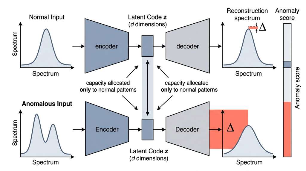
An autoencoder copies its input to its output through a narrow internal bottleneck. This bottleneck forces the network to discover compact features that capture the essence of the training data. Any input whose structure differs from the training data maps poorly onto those learned features, producing a measurable reconstruction gap. The encoder compresses input into fewer dimensions, and the decoder rebuilds the full input from that compressed code. Prefer autoencoders over classical methods (such as Isolation Forest or LOF) when your data is high-dimensional or structured (images, spectra, sequences). They also scale to millions of observations without storing the training set in memory.

More formally, an autoencoder learns two functions: an encoder \(f_\phi: \mathbb{R}^D \to \mathbb{R}^d\) that maps high-dimensional input \(x\) to a low-dimensional latent code \(z = f_\phi(x)\), and a decoder \(g_\theta: \mathbb{R}^d \to \mathbb{R}^D\) that reconstructs the input from the code \(\hat{x} = g_\theta(z)\). Training minimizes the reconstruction loss:

Train the autoencoder on normal data only. The bottleneck learns a compact representation of normal patterns and allocates no capacity to anomalous ones, so anomalous inputs reconstruct poorly. The reconstruction error \(\|x - \hat{x}\|^2\) serves directly as an anomaly score: the larger the gap between input and reconstruction, the less the input resembles the training distribution. In short: if the network cannot rebuild it, the network has never learned anything like it. Figure 30.2.1 illustrates the autoencoder anomaly detection pipeline.

import torch
import torch.nn as nn
import numpy as np

class AnomalyAutoencoder(nn.Module):
    """Autoencoder for anomaly detection with configurable architecture."""

    def __init__(self, input_dim: int, latent_dim: int = 16, hidden_dims: list = None):
        super().__init__()
        if hidden_dims is None:
            hidden_dims = [64, 32]

        # Build encoder
        encoder_layers = []
        prev_dim = input_dim
        for h_dim in hidden_dims:
            encoder_layers.extend([
                nn.Linear(prev_dim, h_dim),
                nn.ReLU(),
                nn.BatchNorm1d(h_dim),
            ])
            prev_dim = h_dim
        encoder_layers.append(nn.Linear(prev_dim, latent_dim))
        self.encoder = nn.Sequential(*encoder_layers)

        # Build decoder (mirror of encoder)
        decoder_layers = []
        prev_dim = latent_dim
        for h_dim in reversed(hidden_dims):
            decoder_layers.extend([
                nn.Linear(prev_dim, h_dim),
                nn.ReLU(),
                nn.BatchNorm1d(h_dim),
            ])
            prev_dim = h_dim
        decoder_layers.append(nn.Linear(prev_dim, input_dim))
        self.decoder = nn.Sequential(*decoder_layers)

    def forward(self, x):
        z = self.encoder(x)
        x_hat = self.decoder(z)
        return x_hat, z

    def anomaly_score(self, x):
        """Reconstruction error as anomaly score."""
        self.eval()
        with torch.no_grad():
            x_hat, _ = self.forward(x)
            scores = torch.mean((x - x_hat) ** 2, dim=1)
        return scores


def train_autoencoder(model, X_train, epochs=100, lr=1e-3, batch_size=64):
    """Train autoencoder on normal data only."""
    optimizer = torch.optim.Adam(model.parameters(), lr=lr)
    dataset = torch.utils.data.TensorDataset(torch.FloatTensor(X_train))
    loader = torch.utils.data.DataLoader(dataset, batch_size=batch_size, shuffle=True)

    model.train()
    for epoch in range(epochs):
        total_loss = 0
        for (batch,) in loader:
            x_hat, _ = model(batch)
            loss = nn.functional.mse_loss(x_hat, batch)
            optimizer.zero_grad()
            loss.backward()
            optimizer.step()
            total_loss += loss.item() * len(batch)
        if (epoch + 1) % 25 == 0:
            print(f"Epoch {epoch+1}/{epochs}, Loss: {total_loss/len(X_train):.6f}")
    return model


# Example: synthetic spectral data (100 wavelength channels)
rng = np.random.default_rng(42)
n_normal, n_anomaly, n_features = 1000, 50, 100

# Normal spectra: smooth Gaussian-like profiles
X_normal = np.zeros((n_normal, n_features))
for i in range(n_normal):
    center = rng.uniform(30, 70)
    width = rng.uniform(5, 15)
    X_normal[i] = np.exp(-0.5 * ((np.arange(n_features) - center) / width) ** 2)
    X_normal[i] += rng.normal(0, 0.02, n_features)  # measurement noise

# Anomalous spectra: double-peaked or sharp emission lines
X_anomaly = np.zeros((n_anomaly, n_features))
for i in range(n_anomaly):
    c1, c2 = rng.uniform(20, 45), rng.uniform(55, 80)
    X_anomaly[i] = 0.5 * np.exp(-0.5 * ((np.arange(n_features) - c1) / 3) ** 2)
    X_anomaly[i] += 0.5 * np.exp(-0.5 * ((np.arange(n_features) - c2) / 3) ** 2)
    X_anomaly[i] += rng.normal(0, 0.02, n_features)

# Train on normal data only (novelty detection setup)
model = AnomalyAutoencoder(input_dim=n_features, latent_dim=8, hidden_dims=[64, 32])
model = train_autoencoder(model, X_normal, epochs=100, lr=1e-3)

# Score both normal and anomalous data
X_all = np.vstack([X_normal, X_anomaly])
labels = np.array([0]*n_normal + [1]*n_anomaly)
scores = model.anomaly_score(torch.FloatTensor(X_all)).numpy()

print(f"\nMean score (normal): {scores[labels==0].mean():.6f}")
print(f"Mean score (anomaly): {scores[labels==1].mean():.6f}")
print(f"Ratio: {scores[labels==1].mean() / scores[labels==0].mean():.1f}x")

Epoch 25/100, Loss: 0.000892
Epoch 50/100, Loss: 0.000531
Epoch 75/100, Loss: 0.000478
Epoch 100/100, Loss: 0.000452

Mean score (normal): 0.000461
Mean score (anomaly): 0.012847
Ratio: 27.9x

2. Variational Autoencoders (VAEs) for Anomaly Scoring

Reconstruction error is a useful anomaly signal, but it tells us nothing about how probable an observation is under a learned model of normality; upgrading from a point estimate to a full probability distribution over latent codes addresses exactly that gap.

Standard autoencoders produce anomaly scores via reconstruction error, but they lack a principled probability model. VAEs (Kingma & Welling, 2014) fix this by learning both an encoder \(q_\phi(z|x)\) that maps inputs to a distribution over latent codes and a decoder \(p_\theta(x|z)\) that generates data from codes. The training objective is the evidence lower bound (ELBO), where the ELBO is a tractable lower bound on the log-likelihood \(\log p(x)\) that can be optimized by gradient descent:

The first term encourages faithful reconstruction (as in standard autoencoders). The second term, the Kullback-Leibler (KL) divergence, pushes the learned posterior \(q_\phi(z|x)\) toward the prior \(p(z) = \mathcal{N}(0, I)\), regularizing the latent space to be smooth and continuous. Because the encoder outputs a distribution rather than a fixed point, sampling from it during training requires the reparameterization trick: instead of sampling \(z\) directly from \(q_\phi(z|x)\), we compute \(z = \mu + \sigma \odot \epsilon\) where \(\epsilon \sim \mathcal{N}(0, I)\), which allows gradients to flow back through \(\mu\) and \(\sigma\) during backpropagation. For anomaly detection, the VAE provides two complementary scores:

Reconstruction probability: \(\log p_\theta(x|z)\) evaluated at the mean of \(q_\phi(z|x)\). Low reconstruction probability indicates the model cannot generate data that looks like the input.

ELBO score: the full ELBO combines reconstruction and regularization. An input that both reconstructs poorly and maps to an unusual region of latent space receives a particularly low ELBO, making this a more robust anomaly score than reconstruction error alone.

In practice, a hyperparameter \(\beta\) is often used to weight the KL term relative to the reconstruction term, giving the loss \(\mathcal{L} = \text{recon} + \beta \cdot D_{\text{KL}}\). Setting \(\beta < 1\) prioritizes reconstruction quality (better anomaly separation by reconstruction error), while \(\beta > 1\) enforces a more structured latent space (better anomaly separation by latent-space distance). This trade-off, known as the \(\beta\)-VAE framework, lets you tune whether the anomaly score relies more on reconstruction fidelity or on latent-space regularity.

class VAEAnomalyDetector(nn.Module):
    """Variational autoencoder for probabilistic anomaly scoring."""

    def __init__(self, input_dim: int, latent_dim: int = 8, hidden_dim: int = 64):
        super().__init__()
        # Encoder: outputs mean and log-variance of q(z|x)
        self.encoder = nn.Sequential(
            nn.Linear(input_dim, hidden_dim), nn.ReLU(),
            nn.Linear(hidden_dim, hidden_dim // 2), nn.ReLU(),
        )
        self.fc_mu = nn.Linear(hidden_dim // 2, latent_dim)
        self.fc_logvar = nn.Linear(hidden_dim // 2, latent_dim)

        # Decoder: p(x|z)
        self.decoder = nn.Sequential(
            nn.Linear(latent_dim, hidden_dim // 2), nn.ReLU(),
            nn.Linear(hidden_dim // 2, hidden_dim), nn.ReLU(),
            nn.Linear(hidden_dim, input_dim),
        )
        self.latent_dim = latent_dim

    def encode(self, x):
        h = self.encoder(x)
        return self.fc_mu(h), self.fc_logvar(h)

    def reparameterize(self, mu, logvar):
        """Reparameterization trick: sample z = mu + sigma * epsilon,
        where epsilon ~ N(0,I), so gradients flow through mu and sigma."""
        std = torch.exp(0.5 * logvar)
        eps = torch.randn_like(std)
        return mu + eps * std

    def forward(self, x):
        mu, logvar = self.encode(x)
        z = self.reparameterize(mu, logvar)
        x_hat = self.decoder(z)
        return x_hat, mu, logvar

    def elbo_anomaly_score(self, x, n_samples: int = 10):
        """Negative ELBO as anomaly score (higher = more anomalous)."""
        self.eval()
        with torch.no_grad():
            mu, logvar = self.encode(x)
            # Monte Carlo estimate of reconstruction term
            recon_loss = 0
            for _ in range(n_samples):
                z = self.reparameterize(mu, logvar)
                x_hat = self.decoder(z)
                recon_loss += torch.sum((x - x_hat) ** 2, dim=1)
            recon_loss /= n_samples
            # KL divergence: closed form for Gaussian
            kl_div = -0.5 * torch.sum(1 + logvar - mu**2 - logvar.exp(), dim=1)
            return recon_loss + kl_div  # negative ELBO


def train_vae(model, X_train, epochs=150, lr=1e-3, batch_size=64, beta=1.0):
    """Train VAE with optional beta-weighting on KL term."""
    optimizer = torch.optim.Adam(model.parameters(), lr=lr)
    dataset = torch.utils.data.TensorDataset(torch.FloatTensor(X_train))
    loader = torch.utils.data.DataLoader(dataset, batch_size=batch_size, shuffle=True)

    model.train()
    for epoch in range(epochs):
        total_loss = 0
        for (batch,) in loader:
            x_hat, mu, logvar = model(batch)
            recon = nn.functional.mse_loss(x_hat, batch, reduction='sum')
            kl = -0.5 * torch.sum(1 + logvar - mu**2 - logvar.exp())
            loss = recon + beta * kl
            optimizer.zero_grad()
            loss.backward()
            optimizer.step()
            total_loss += loss.item()
        if (epoch + 1) % 50 == 0:
            print(f"Epoch {epoch+1}/{epochs}, Loss: {total_loss/len(X_train):.4f}")
    return model


# Train VAE on normal spectra
vae = VAEAnomalyDetector(input_dim=n_features, latent_dim=8, hidden_dim=64)
vae = train_vae(vae, X_normal, epochs=150, lr=1e-3, beta=0.5)

# Score with ELBO
vae_scores = vae.elbo_anomaly_score(torch.FloatTensor(X_all), n_samples=20).numpy()
print(f"\nVAE ELBO score (normal): {vae_scores[labels==0].mean():.4f}")
print(f"VAE ELBO score (anomaly): {vae_scores[labels==1].mean():.4f}")
print(f"Separation ratio: {vae_scores[labels==1].mean() / vae_scores[labels==0].mean():.1f}x")

3. Normalizing Flows for Exact Likelihood

The ELBO that VAEs optimize is, by definition, a lower bound on the true log-likelihood; the gap between the bound and the exact value means that some anomalies may receive scores that are off by an unknown margin. Normalizing flows close that gap entirely.

Both autoencoders and VAEs provide proxy scores for anomalies (reconstruction error or ELBO bound). Normalizing flows (Rezende & Mohamed, 2015), where a "flow" is a chain of invertible neural network layers that together define a bijective mapping between data space and latent space, offer something stronger: exact computation of the log-likelihood \(\log p(x)\) under a learned generative model. If \(\log p(x)\) is low, the observation is genuinely improbable under the model, which is among the most principled definitions of an anomaly.

A normalizing flow defines an invertible transformation \(f: \mathbb{R}^D \to \mathbb{R}^D\) that maps a simple base distribution \(p_z(z) = \mathcal{N}(0, I)\) to the complex data distribution \(p_x(x)\). By the change of variables formula:

Mental Model

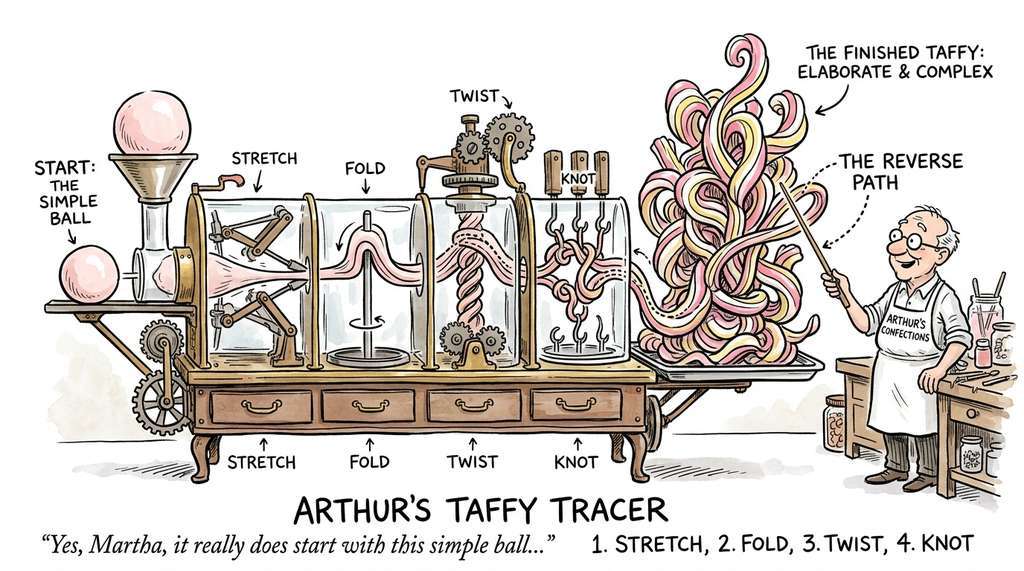
Think of a normalizing flow like a taffy-pulling machine. You start with a simple, uniform ball of taffy (the Gaussian base distribution) and apply a series of precise stretches, folds, and twists (the invertible transformations) until the taffy takes a complex final shape that matches your data. Because every stretch is reversible, you can take any piece of the finished taffy and trace it back through every step to find exactly where it came from in the original ball. Points that trace back to the dense center of the original ball are common; points that trace back to the far edge are rare. The Jacobian determinant, where the Jacobian is the matrix of all partial derivatives of the transformation, accounts for how much each stretch thinned or thickened the taffy at that spot, letting you compute exact density everywhere.

The first term measures how likely the transformed point is under the base distribution. The second term (the log-determinant of the Jacobian) accounts for how the transformation stretches or compresses local volume. Training maximizes the total log-likelihood over the training data. At test time, low \(\log p_x(x)\) indicates an anomaly.

class RealNVPCoupling(nn.Module):
    """Single coupling layer for a RealNVP normalizing flow.

    RealNVP (Real-valued Non-Volume Preserving) splits dimensions into
    two groups: one group passes through unchanged, while the other is
    scaled and translated by neural networks conditioned on the first group.
    """

    def __init__(self, dim: int, hidden_dim: int = 64, mask_type: str = 'even'):
        super().__init__()
        self.dim = dim
        # Binary mask: which dimensions are transformed vs. passed through
        if mask_type == 'even':
            self.register_buffer('mask', torch.arange(dim).float() % 2)
        else:
            self.register_buffer('mask', 1 - torch.arange(dim).float() % 2)

        # Scale and translate networks
        self.scale_net = nn.Sequential(
            nn.Linear(dim, hidden_dim), nn.ReLU(),
            nn.Linear(hidden_dim, hidden_dim), nn.ReLU(),
            nn.Linear(hidden_dim, dim), nn.Tanh(),  # bounded scale
        )
        self.translate_net = nn.Sequential(
            nn.Linear(dim, hidden_dim), nn.ReLU(),
            nn.Linear(hidden_dim, hidden_dim), nn.ReLU(),
            nn.Linear(hidden_dim, dim),
        )

    def forward(self, x):
        """Forward: data -> latent. Returns transformed x and log-det-jacobian."""
        x_masked = x * self.mask
        s = self.scale_net(x_masked) * (1 - self.mask)
        t = self.translate_net(x_masked) * (1 - self.mask)
        y = x_masked + (1 - self.mask) * (x * torch.exp(s) + t)
        log_det = s.sum(dim=1)
        return y, log_det

    def inverse(self, y):
        """Inverse: latent -> data."""
        y_masked = y * self.mask
        s = self.scale_net(y_masked) * (1 - self.mask)
        t = self.translate_net(y_masked) * (1 - self.mask)
        x = y_masked + (1 - self.mask) * (y - t) * torch.exp(-s)
        return x


class RealNVPFlow(nn.Module):
    """RealNVP normalizing flow for density estimation and anomaly detection."""

    def __init__(self, dim: int, n_layers: int = 6, hidden_dim: int = 64):
        super().__init__()
        self.layers = nn.ModuleList()
        for i in range(n_layers):
            mask_type = 'even' if i % 2 == 0 else 'odd'
            self.layers.append(RealNVPCoupling(dim, hidden_dim, mask_type))
        self.dim = dim

    def forward(self, x):
        """Map data to latent space, accumulating log-det-jacobian."""
        log_det_total = torch.zeros(x.shape[0], device=x.device)
        z = x
        for layer in self.layers:
            z, log_det = layer(z)
            log_det_total += log_det
        return z, log_det_total

    def log_prob(self, x):
        """Exact log-likelihood under the flow model."""
        z, log_det = self.forward(x)
        # Log-prob under base distribution (standard normal)
        log_pz = -0.5 * (z**2 + np.log(2 * np.pi)).sum(dim=1)
        return log_pz + log_det

    def anomaly_score(self, x):
        """Negative log-likelihood as anomaly score."""
        self.eval()
        with torch.no_grad():
            return -self.log_prob(x)


def train_flow(model, X_train, epochs=200, lr=1e-3, batch_size=64):
    """Train normalizing flow by maximum likelihood."""
    optimizer = torch.optim.Adam(model.parameters(), lr=lr)
    dataset = torch.utils.data.TensorDataset(torch.FloatTensor(X_train))
    loader = torch.utils.data.DataLoader(dataset, batch_size=batch_size, shuffle=True)

    model.train()
    for epoch in range(epochs):
        total_nll = 0
        for (batch,) in loader:
            nll = -model.log_prob(batch).mean()  # negative log-likelihood
            optimizer.zero_grad()
            nll.backward()
            optimizer.step()
            total_nll += nll.item() * len(batch)
        if (epoch + 1) % 50 == 0:
            print(f"Epoch {epoch+1}/{epochs}, NLL: {total_nll/len(X_train):.4f}")
    return model


# Train flow on normal spectra
flow = RealNVPFlow(dim=n_features, n_layers=8, hidden_dim=64)
flow = train_flow(flow, X_normal, epochs=200, lr=5e-4)

# Score all data with exact log-likelihood
flow_scores = flow.anomaly_score(torch.FloatTensor(X_all)).numpy()
print(f"\nFlow NLL (normal): {flow_scores[labels==0].mean():.2f}")
print(f"Flow NLL (anomaly): {flow_scores[labels==1].mean():.2f}")

4. Out-of-Distribution Detection for Neural Networks

The generative methods above learn what normal data looks like and flag deviations; but in supervised settings, we face a complementary problem: a trained classifier that encounters data entirely outside its training domain may still produce a confident (and meaningless) prediction.

Out-of-distribution (OOD) detection, where "out-of-distribution" means the input comes from a different data-generating process than the one represented in the training set, addresses a specific failure mode of supervised neural networks: producing confident predictions on inputs that bear no relation to the training data. A classifier trained on chest X-rays should not return a confident diagnosis when given a photograph of a cat, yet standard softmax classifiers (where the softmax function converts raw network outputs into a probability distribution that sums to one) will do exactly that. OOD detection adds a safety layer that flags inputs the model should refuse to classify.

Post-hoc Detection Scores

The Maximum Softmax Probability (MSP) baseline (Hendrycks & Gimpel, 2017) uses the maximum of the softmax output as a confidence score. In-distribution inputs tend to produce high MSP; OOD inputs tend to produce lower MSP, though the separation is often poor. ODIN (Liang et al., 2018) improves on MSP with two modifications. First, it computes softmax at temperature \(T > 1\), spreading the distribution and amplifying differences. Second, it perturbs inputs in the direction that increases the maximum softmax probability. This perturbation benefits in-distribution inputs more than OOD inputs, widening the gap between the two.

More recent methods operate in the feature space rather than the output space. Mahalanobis distance (Lee et al., 2018) fits a class-conditional Gaussian to the penultimate layer features and scores inputs by their Mahalanobis distance (a distance metric that accounts for correlations between features by weighting differences through the inverse covariance matrix) to the nearest class centroid. Energy-based scoring (Liu et al., 2020) uses the negative log of the partition function (the normalizing constant in the denominator of the softmax, which sums the exponentiated logits across all classes) as a theoretically grounded OOD score:

where \(f_c(x)\) is the logit (the raw, unnormalized output of the network's final layer before the softmax transformation) for class \(c\). Low energy (high partition function) indicates in-distribution; high energy indicates OOD. (As of 2024, newer post-hoc OOD scorers such as Virtual-logit Matching (ViM; Wang et al., 2022), KNN-based detection (Sun et al., 2022), and Activation Shaping (ASH; Djurisic et al., 2023) often outperform energy scoring on standard benchmarks while remaining equally simple to apply to a pretrained classifier.)

import torch.nn.functional as F

def energy_score(logits: torch.Tensor, temperature: float = 1.0) -> torch.Tensor:
    """Energy-based OOD score: -T * log(sum(exp(logits/T))).

    Lower energy = more likely in-distribution.
    Higher energy = more likely OOD.
    """
    return -temperature * torch.logsumexp(logits / temperature, dim=1)


def mahalanobis_ood_score(features: torch.Tensor,
                          class_means: list[torch.Tensor],
                          precision: torch.Tensor) -> torch.Tensor:
    """Mahalanobis distance to nearest class centroid in feature space.

    Args:
        features: (N, D) feature vectors from penultimate layer
        class_means: list of (D,) class centroid vectors
        precision: (D, D) shared precision matrix (inverse covariance)
    Returns:
        (N,) minimum Mahalanobis distance across classes
    """
    min_distances = torch.full((features.shape[0],), float('inf'))
    for mu in class_means:
        diff = features - mu.unsqueeze(0)  # (N, D)
        # Mahalanobis: sqrt(diff @ precision @ diff^T), squared for efficiency
        m_dist = torch.sum(diff @ precision * diff, dim=1)
        min_distances = torch.minimum(min_distances, m_dist)
    return min_distances


# Example: comparing MSP and energy scores on a trained classifier
# Assume 'classifier' is a trained model, 'in_loader' and 'ood_loader' are data loaders
# (Pseudocode showing the evaluation pattern)
"""
in_energies, ood_energies = [], []
for x, _ in in_loader:
    logits = classifier(x)
    in_energies.append(energy_score(logits))
for x, _ in ood_loader:
    logits = classifier(x)
    ood_energies.append(energy_score(logits))

in_energies = torch.cat(in_energies)
ood_energies = torch.cat(ood_energies)
# AUROC: how well does the energy score separate in-dist from OOD?
auroc = compute_auroc(in_energies, ood_energies)
"""

from openood.evaluators import OODEvaluator

evaluator = OODEvaluator(model, id_data='cifar10', ood_data=['svhn', 'textures'])
results = evaluator.evaluate(methods=['msp', 'energy', 'mahalanobis'])
# Returns AUROC, FPR@95TPR, and detection accuracy for each method

Exercises

1. (Conceptual) An autoencoder trained on normal electrocardiogram (ECG) signals achieves low reconstruction error on atrial fibrillation episodes. Explain why this might happen (hint: consider the latent dimension and training data diversity). How would you modify the architecture or training procedure to improve anomaly detection for this case?
2. (Coding) Implement all three deep anomaly detectors (autoencoder, VAE, normalizing flow) on the PyOD cardio dataset. Compare their AUROC scores and training times. Which method provides the best score separation? Plot the score distributions for normal and anomalous classes for each method.
3. (Analysis) The "typicality" problem (Nalisnick et al., 2019) shows that high likelihood does not guarantee in-distribution. Implement a likelihood ratio test by training two normalizing flows: one on your target data and one on a generic reference dataset. Show that the ratio \(\log p_{\text{target}}(x) - \log p_{\text{reference}}(x)\) provides better OOD separation than raw likelihood alone. Use synthetic data to construct a clear demonstration.