30.3 Drift and Open-World Learning

1. Data Drift vs. Concept Drift

Your sensor readings shift by two degrees over six months: should you retrain your model, recalibrate the instrument, or publish a discovery paper? The answer depends entirely on which flavor of drift you are facing, and conflating them leads to the wrong response every time.

Data drift (also called covariate shift, meaning the distribution of input features changes while the target relationship holds) means the input distribution \(P(X)\) has changed while the relationship between inputs and outputs \(P(Y|X)\) remains the same. If a weather station's thermometer develops a systematic bias of +2 degrees, all temperature readings shift, but the relationship between temperature and atmospheric pressure is unchanged. Data drift requires recalibrating inputs, not retraining models.

Data drift is the most frequent distributional change in deployed systems, yet it does not invalidate your learned model. The mechanism: something upstream (a sensor, a sampling procedure, a population demographic) shifts the marginal distribution of features, while the causal relationship between features and targets stays intact. Suspect data drift rather than concept drift when model accuracy degrades but domain experts confirm the underlying science has not changed. The correct response is input recalibration or feature-level normalization, not a full retrain. Retraining on pure covariate shift wastes compute and risks introducing unnecessary variance.

Concept drift means the relationship \(P(Y|X)\) itself has changed. The same input now maps to a different output. In fraud detection, a transaction pattern that was legitimate last year might signal fraud this year because criminal tactics have evolved. In drug discovery, a molecular fingerprint that predicted activity against one viral variant may not predict activity against a new variant. Concept drift requires retraining or adapting the model. In short: data drift moves the inputs; concept drift rewrites the rules.

In scientific contexts, a third category deserves attention: discovery drift, where the underlying phenomenon genuinely changes. Climate data exhibits discovery drift as global temperatures rise; the "normal" baseline is a moving target. Astronomical surveys exhibit discovery drift as new types of transient events (kilonovae, fast radio bursts) are recognized. Discovery drift is the most scientifically interesting form: it signals that the world itself has changed, not just our measurement of it. Figure 30.4 summarizes all three drift types, their defining characteristics, and the correct response for each.

2. CUSUM: The Classical Change-Point Detector

Knowing the difference between data drift and concept drift is only useful if you can detect the moment a shift begins; the next question is how to build a detector that raises an alarm as quickly as possible after the distribution changes.

The Cumulative Sum (CUSUM) control chart (Page, 1954) is the most theoretically grounded change-point detector. Over 70 years after its introduction, it typically remains competitive for detecting mean shifts in univariate streams (a property demonstrated by comparative studies such as Lu et al., 2019, which benchmark it against modern alternatives), and its simplicity keeps it a staple in production systems.

Given a stream of observations \(x_1, x_2, \ldots\) with expected mean \(\mu_0\) under the null hypothesis (no drift), CUSUM maintains two statistics that track cumulative deviations above and below the expected mean:

where \(k\) is the allowance parameter (slack) that prevents the statistic from drifting upward due to random fluctuations. A drift alarm fires when either \(S_t^+\) or \(S_t^-\) exceeds a threshold \(h\). The parameters \(k\) and \(h\) control the trade-off between detection delay and false alarm rate: smaller \(k\) and \(h\) detect smaller shifts faster but produce more false alarms.

For a shift of magnitude \(\delta\) in the mean, the optimal allowance is \(k = \delta/2\) (halfway between the old and new mean). In practice, when the shift magnitude is unknown, \(k\) is set to half the smallest shift worth detecting.

import numpy as np

class CUSUM:
    """CUSUM change-point detector for univariate streams.

    Detects shifts in the mean of a stream relative to a reference value.
    """

    def __init__(self, target_mean: float, allowance: float, threshold: float):
        self.target_mean = target_mean
        self.k = allowance   # slack parameter
        self.h = threshold   # alarm threshold
        self.s_pos = 0.0     # upper CUSUM statistic
        self.s_neg = 0.0     # lower CUSUM statistic
        self.t = 0           # observation counter
        self.alarm_times = []

    def update(self, x: float) -> bool:
        """Process one observation. Returns True if drift is detected."""
        self.t += 1
        deviation = x - self.target_mean
        self.s_pos = max(0, self.s_pos + deviation - self.k)
        self.s_neg = max(0, self.s_neg - deviation - self.k)

        if self.s_pos > self.h or self.s_neg > self.h:
            self.alarm_times.append(self.t)
            self.s_pos = 0  # reset after alarm
            self.s_neg = 0
            return True
        return False

    def run(self, stream: np.ndarray) -> list[int]:
        """Process entire stream, return list of alarm times."""
        alarms = []
        for i, x in enumerate(stream):
            if self.update(x):
                alarms.append(i)
        return alarms


# Simulate a scientific measurement stream with a mid-experiment drift
rng = np.random.default_rng(42)
n_before, n_after = 500, 500
sigma = 1.0
shift = 1.5  # the drift magnitude

# Phase 1: stable measurements around mean=10
stream_stable = rng.normal(loc=10.0, scale=sigma, size=n_before)
# Phase 2: drifted measurements around mean=11.5
stream_drifted = rng.normal(loc=10.0 + shift, scale=sigma, size=n_after)
stream = np.concatenate([stream_stable, stream_drifted])

# Configure CUSUM: allowance = shift/2, threshold tuned for ~1% false alarm rate
detector = CUSUM(target_mean=10.0, allowance=shift/2, threshold=5.0)
alarms = detector.run(stream)

print(f"True change point: t={n_before}")
print(f"Alarm times: {alarms}")
if alarms:
    first_alarm = alarms[0]
    detection_delay = first_alarm - n_before
    print(f"Detection delay: {detection_delay} observations")
    print(f"Correct detection: {first_alarm > n_before - 10}")  # within reasonable margin

True change point: t=500
Alarm times: [511]
Detection delay: 11 observations
Correct detection: True

3. Modern Drift Detectors

CUSUM works well for univariate mean shifts, but scientific data often requires more flexible drift detection. Three modern methods extend CUSUM's core idea to handle different scenarios.

ADWIN (Adaptive Windowing; Bifet & Gavalda, 2007) maintains a variable-length window of recent observations and tests whether any partition of this window into two sub-windows shows a statistically significant difference in means. Unlike CUSUM, ADWIN requires no prior specification of the expected mean or shift magnitude; it adapts automatically. The window grows during stable periods (accumulating evidence) and shrinks when drift is detected (forgetting outdated data).

Page-Hinkley (Page, 1954; Hinkley, 1971) is a close relative of CUSUM that monitors the running mean directly. It computes the cumulative deviation of observations from their running mean and fires an alarm when this deviation exceeds a threshold. Page-Hinkley is often more intuitive to tune than CUSUM because its threshold has a direct interpretation as the maximum tolerable cumulative deviation.

DDM (Drift Detection Method; Gama et al., 2004) monitors the error rate of a supervised model and flags drift when the error rate increases significantly relative to its historical minimum. DDM distinguishes between "warning" (possible drift) and "alarm" (confirmed drift) levels, allowing gradual model adaptation. It is particularly useful for monitoring deployed classifiers in production, the MLOps use case of Chapter 22.

from river import drift

# Compare three drift detectors on the same stream
detectors = {
    'ADWIN': drift.ADWIN(delta=0.002),
    'PageHinkley': drift.PageHinkley(
        min_instances=30, delta=0.005, threshold=50, alpha=0.9999
    ),
}

results = {}
for name, detector in detectors.items():
    alarms = []
    for i, x in enumerate(stream):
        detector.update(x)
        if detector.drift_detected:
            alarms.append(i)
    results[name] = alarms
    print(f"{name}: alarms at {alarms[:5]}")  # show first 5

# Our custom CUSUM for comparison
print(f"CUSUM: alarms at {alarms[:5]}")
print(f"\nTrue change point: t={n_before}")

from river.drift import ADWIN
detector = ADWIN(delta=0.002)
for x in stream:
    detector.update(x)
    if detector.drift_detected:
        print(f"Drift at observation {detector.n}")

4. Multivariate and High-Dimensional Drift

Running a separate univariate detector on each of a spectrometer's 500 channels produces hundreds of independent alarms, most of them false positives from multiple testing, while completely missing drift patterns that only appear in the correlations between channels. Multivariate drift tests solve both problems at once.

Scientific instruments often produce multivariate streams: a mass spectrometer outputs intensity across hundreds of mass-to-charge ratios simultaneously; a genomics pipeline produces expression values for thousands of genes per sample. Univariate drift detectors applied independently to each dimension miss correlated shifts and suffer from multiple-testing problems.

Maximum Mean Discrepancy (MMD) provides a principled multivariate test for distributional differences. Given samples from two distributions \(P\) and \(Q\), MMD measures the distance between their embeddings in a reproducing kernel Hilbert space (RKHS), where RKHS is a function space in which every point evaluation is a continuous linear functional, allowing distributions to be compared via their mean embeddings:

where \(x, x' \sim P\), \(y, y' \sim Q\), and \(k\) is a kernel function (typically radial basis function (RBF)). Under the null hypothesis \(P = Q\), \(\text{MMD}^2 = 0\). A permutation test (a nonparametric significance test that repeatedly shuffles group labels to build a null distribution of the test statistic) or asymptotic approximation provides p-values. For streaming data, a sliding-window variant compares recent observations to a reference window.

def mmd_squared(X: np.ndarray, Y: np.ndarray, gamma: float = 1.0) -> float:
    """Compute squared Maximum Mean Discrepancy with RBF kernel.

    Args:
        X: (n, d) samples from distribution P
        Y: (m, d) samples from distribution Q
        gamma: RBF kernel bandwidth parameter
    Returns:
        Squared MMD statistic
    """
    def rbf_kernel(A, B, gamma):
        # ||a - b||^2 = ||a||^2 + ||b||^2 - 2 a.b
        sq_a = np.sum(A**2, axis=1, keepdims=True)
        sq_b = np.sum(B**2, axis=1, keepdims=True)
        dist_sq = sq_a + sq_b.T - 2 * A @ B.T
        return np.exp(-gamma * dist_sq)

    K_xx = rbf_kernel(X, X, gamma)
    K_yy = rbf_kernel(Y, Y, gamma)
    K_xy = rbf_kernel(X, Y, gamma)

    n, m = len(X), len(Y)
    # Unbiased estimate: exclude diagonal terms
    mmd2 = (K_xx.sum() - np.trace(K_xx)) / (n * (n - 1))
    mmd2 += (K_yy.sum() - np.trace(K_yy)) / (m * (m - 1))
    mmd2 -= 2 * K_xy.sum() / (n * m)
    return mmd2


def mmd_permutation_test(X: np.ndarray, Y: np.ndarray,
                         gamma: float = 1.0, n_permutations: int = 500) -> tuple:
    """Two-sample test: are X and Y from the same distribution?"""
    observed_mmd = mmd_squared(X, Y, gamma)

    # Permutation null distribution
    combined = np.vstack([X, Y])
    n = len(X)
    null_mmds = np.zeros(n_permutations)
    rng = np.random.default_rng(42)

    for i in range(n_permutations):
        perm = rng.permutation(len(combined))
        X_perm = combined[perm[:n]]
        Y_perm = combined[perm[n:]]
        null_mmds[i] = mmd_squared(X_perm, Y_perm, gamma)

    p_value = (null_mmds >= observed_mmd).mean()
    return observed_mmd, p_value


# Example: detect multivariate drift in 10-dimensional sensor data
rng = np.random.default_rng(42)
d = 10
reference = rng.multivariate_normal(np.zeros(d), np.eye(d), size=200)

# Test 1: same distribution (no drift)
test_same = rng.multivariate_normal(np.zeros(d), np.eye(d), size=200)
mmd_val, p_val = mmd_permutation_test(reference, test_same)
print(f"No drift:  MMD^2 = {mmd_val:.6f}, p = {p_val:.3f}")

# Test 2: mean shift in 3 dimensions (subtle multivariate drift)
shifted_mean = np.zeros(d)
shifted_mean[:3] = 0.5  # shift first 3 dimensions by 0.5 sigma
test_shifted = rng.multivariate_normal(shifted_mean, np.eye(d), size=200)
mmd_val, p_val = mmd_permutation_test(reference, test_shifted)
print(f"Subtle drift: MMD^2 = {mmd_val:.6f}, p = {p_val:.3f}")

# Test 3: covariance change (no mean shift)
cov_changed = np.eye(d)
cov_changed[:3, :3] = [[1, 0.8, 0.8], [0.8, 1, 0.8], [0.8, 0.8, 1]]
test_cov = rng.multivariate_normal(np.zeros(d), cov_changed, size=200)
mmd_val, p_val = mmd_permutation_test(reference, test_cov)
print(f"Cov drift:   MMD^2 = {mmd_val:.6f}, p = {p_val:.3f}")

No drift:  MMD^2 = -0.000312, p = 0.616
Subtle drift: MMD^2 = 0.023841, p = 0.000
Cov drift:   MMD^2 = 0.048976, p = 0.000

5. Open-World Learning

Drift detectors tell us when the data distribution has changed, but they say nothing about what has appeared; when the shift is caused by an entirely new phenomenon rather than a gradual slide in familiar quantities, we need a framework that can recognize the unknown as unknown.

Standard classification assumes a closed world: every test input belongs to one of the \(C\) classes seen during training. Open-world learning (Bendale & Boult, 2015) relaxes this assumption, allowing the system to recognize inputs from unknown classes and, optionally, learn to classify them incrementally.

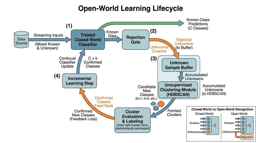
Open-world learning combines three capabilities:

• Reject unknown: correctly identify that an input does not belong to any known class (the out-of-distribution (OOD) detection problem from Section 30.2).
• Cluster unknown: group rejected inputs into coherent clusters that might represent new classes.
• Learn incrementally: incorporate confirmed new classes into the classifier without catastrophic forgetting, where catastrophic forgetting is the tendency of neural networks to abruptly lose previously learned knowledge when trained on new data. Figure 30.3.1 illustrates open-world learning lifecycle.

These three capabilities mirror what scientists do naturally: encounter something that does not fit existing categories, collect more examples, and define a new category. The transition from rejection to clustering to incremental learning forms a pipeline, where each stage feeds the next. Fast radio bursts (FRBs) in radio astronomy illustrate this process. Researchers initially classified the first FRB (Lorimer et al., 2007) as interference. Only after they collected, clustered, and confirmed multiple examples as astrophysical did "FRB" become a recognized transient class.

from sklearn.metrics import pairwise_distances
from collections import defaultdict

class OpenWorldClassifier:
    """Simple open-world classifier: known-class centroids + rejection threshold."""

    def __init__(self, rejection_threshold: float = 2.0):
        self.rejection_threshold = rejection_threshold
        self.class_centroids = {}   # class_id -> centroid vector
        self.class_radii = {}       # class_id -> max observed distance from centroid
        self.unknown_buffer = []    # buffer of rejected samples for clustering

    def fit(self, X: np.ndarray, y: np.ndarray):
        """Learn centroids and radii from training data."""
        for cls in np.unique(y):
            mask = y == cls
            centroid = X[mask].mean(axis=0)
            distances = np.linalg.norm(X[mask] - centroid, axis=1)
            self.class_centroids[cls] = centroid
            self.class_radii[cls] = distances.max()
        return self

    def predict(self, X: np.ndarray) -> np.ndarray:
        """Predict class or 'unknown' (-1) for each input."""
        predictions = np.full(len(X), -1)  # default: unknown
        for i, x in enumerate(X):
            min_dist, best_cls = float('inf'), -1
            for cls, centroid in self.class_centroids.items():
                dist = np.linalg.norm(x - centroid)
                normalized = dist / self.class_radii[cls]
                if normalized < min_dist:
                    min_dist = normalized
                    best_cls = cls
            if min_dist < self.rejection_threshold:
                predictions[i] = best_cls
            else:
                self.unknown_buffer.append(x)
        return predictions

    def discover_new_classes(self, min_cluster_size: int = 5):
        """Cluster unknown buffer to discover potential new classes."""
        if len(self.unknown_buffer) < min_cluster_size:
            return {}

        from hdbscan import HDBSCAN
        X_unknown = np.array(self.unknown_buffer)
        clusterer = HDBSCAN(min_cluster_size=min_cluster_size)
        labels = clusterer.fit_predict(X_unknown)

        new_classes = {}
        for label in set(labels):
            if label == -1:
                continue  # skip noise
            mask = labels == label
            cluster_data = X_unknown[mask]
            new_class_id = max(self.class_centroids.keys()) + 1 + label
            new_classes[new_class_id] = {
                'centroid': cluster_data.mean(axis=0),
                'size': mask.sum(),
                'samples': cluster_data,
            }
        return new_classes

    def incorporate_class(self, class_id: int, X_new: np.ndarray) -> None:
        """Incorporate a confirmed new class into the classifier.

        This completes the open-world loop: after domain experts confirm
        that a discovered cluster represents a genuine new class, add it
        to the known classes so future instances are classified directly.
        """
        centroid = X_new.mean(axis=0)
        distances = np.linalg.norm(X_new - centroid, axis=1)
        self.class_centroids[class_id] = centroid
        self.class_radii[class_id] = distances.max()
        # Clear incorporated samples from the unknown buffer
        self.unknown_buffer = [
            x for x in self.unknown_buffer
            if np.linalg.norm(x - centroid) > self.class_radii[class_id]
        ]


# Example: 3 known classes, 1 novel class emerging
rng = np.random.default_rng(42)
n_per_class, d = 100, 5

# Known classes
X_train = np.vstack([
    rng.normal(loc=[0,0,0,0,0], scale=0.5, size=(n_per_class, d)),
    rng.normal(loc=[3,3,0,0,0], scale=0.5, size=(n_per_class, d)),
    rng.normal(loc=[0,0,3,3,0], scale=0.5, size=(n_per_class, d)),
])
y_train = np.array([0]*n_per_class + [1]*n_per_class + [2]*n_per_class)

# Test: mix of known classes + novel class
X_test_known = np.vstack([
    rng.normal(loc=[0,0,0,0,0], scale=0.5, size=(30, d)),
    rng.normal(loc=[3,3,0,0,0], scale=0.5, size=(30, d)),
])
X_test_novel = rng.normal(loc=[5,0,5,0,5], scale=0.4, size=(25, d))  # new class!
X_test = np.vstack([X_test_known, X_test_novel])

# Train and predict
owc = OpenWorldClassifier(rejection_threshold=1.8)
owc.fit(X_train, y_train)
preds = owc.predict(X_test)

n_known_correct = (preds[:60] != -1).sum()
n_novel_rejected = (preds[60:] == -1).sum()
print(f"Known samples classified: {n_known_correct}/60")
print(f"Novel samples rejected: {n_novel_rejected}/25")
print(f"Unknown buffer size: {len(owc.unknown_buffer)}")

# Discover new classes from rejected samples
new_classes = owc.discover_new_classes(min_cluster_size=5)
for cls_id, info in new_classes.items():
    print(f"Discovered class {cls_id}: {info['size']} samples, "
          f"centroid mean = {info['centroid'].mean():.2f}")

    # Close the loop: incorporate the confirmed new class
    owc.incorporate_class(cls_id, info['samples'])
    print(f"  -> Incorporated as known class {cls_id} "
          f"(total known classes: {len(owc.class_centroids)})")

Exercises

1. (Conceptual) A genomics pipeline monitors the GC content distribution of sequencing reads. Over three months, the distribution gradually shifts toward higher GC content. Is this data drift, concept drift, or discovery drift? What are three plausible explanations, and what additional data would you collect to distinguish them?
2. (Coding) Implement a streaming drift detection system that combines CUSUM (for mean shifts), a variance monitor (for scale changes), and MMD (for multivariate distributional changes). Test it on a synthetic stream with (a) a sudden mean shift, (b) a gradual variance increase, and (c) a change in correlation structure without any marginal changes. Which detector fires first in each case?
3. (Analysis) The OpenWorldClassifier in Listing 30.12 uses Euclidean distance to centroids for rejection. Replace it with Mahalanobis distance (using each class's covariance matrix) and compare the rejection accuracy on datasets where classes have different shapes (spherical vs. elongated). Under what conditions does Mahalanobis distance substantially outperform Euclidean distance?