Prerequisites
The pipeline below requires familiarity with the classical detectors from Section 30.1 (Local Outlier Factor (LOF), Hierarchical Density-Based Spatial Clustering of Applications with Noise (HDBSCAN), Isolation Forest), the deep methods from Section 30.2 (autoencoders, Variational Autoencoders (VAEs)), and the drift detection concepts from Section 30.3. We also draw on the data pipeline architecture from Chapter 6 and the evaluation methodology from Chapter 22: MLOps.
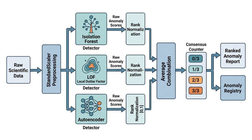
In practice, no single anomaly detection method dominates across all data types and anomaly patterns. LOF catches local density anomalies that Isolation Forest misses. Isolation Forest catches high-dimensional anomalies that Kernel Density Estimation (KDE) cannot handle. Autoencoders catch structural anomalies invisible to all tabular methods. The solution is an ensemble pipeline: run multiple detectors with complementary assumptions, combine their scores, and rank anomalies by consensus. This section builds exactly that pipeline, end to end, from raw data ingestion through consensus scoring to ground-truth validation. The result is a reusable component for the Discovery Workbench (the modular scientific workflow platform introduced in Chapter 6) that can be deployed in any scientific domain. Figure 30.4.1 illustrates three-method ensemble anomaly detection pipeline with rank normalization and consensus scoring.
1. The Three-Method Ensemble Strategy
Imagine a telescope survey flags a faint transient. Isolation Forest scores it as the night's top anomaly, yet LOF ranks it as perfectly ordinary, and an autoencoder reconstructs it with almost zero error. Is that transient a genuine astrophysical event or an instrumental glitch? The answer depends on which detector you trust. If you can only trust one, you will be wrong far too often. The solution is deliberate diversity: combine three methods chosen for complementary strengths so that no single blind spot dictates the outcome.
- Isolation Forest: a tree-based method that detects anomalies through ease of isolation. It makes no density assumptions, scales linearly, and handles high-dimensional data naturally. Its blind spot is anomalies near cluster boundaries.
- LOF (Local Outlier Factor): a density-based method that detects local anomalies by comparing each point's density to its neighbors'. It excels at finding anomalies in datasets with clusters of varying density. Its blind spot is global anomalies in uniformly distributed data.
- Autoencoder reconstruction error: a deep method that detects anomalies through learned data representations. It captures structural and nonlinear patterns invisible to distance-based methods. Its blind spot is anomalies that the network can reconstruct well (when the bottleneck is too wide).
Each method scores anomalies on a different scale. To combine them meaningfully, we need score normalization. The standard approach is to convert each method's raw scores to a common scale using one of three strategies:
Rank normalization: replace each score with its rank divided by the number of samples. This is the most robust option because it is invariant to the score distribution shape. A point ranked 5th out of 1,000 by Isolation Forest and 3rd out of 1,000 by LOF receives normalized scores of 0.005 and 0.003 regardless of the raw score magnitudes.
Rank normalization converts each detector's raw anomaly scores into a uniform distribution on \([0, 1]\) by replacing each score with its fractional position in the sorted order. This step is essential because raw scores from different detectors live on incomparable scales: Isolation Forest might output values near \(-0.5\), LOF might output values near 1.2, and an autoencoder might output reconstruction errors near 0.01. Averaging these raw numbers lets whichever detector produces the largest magnitudes dominate the ensemble. The procedure is straightforward: sort the \(n\) scores, assign each its rank (1 through \(n\)), then divide by \(n - 1\). The least anomalous point maps to 0 and the most anomalous maps to 1. Prefer rank normalization over min-max or z-score alternatives when score distributions are skewed, heavy-tailed, or contain extreme outliers, the typical case for anomaly scores. Reserve z-score normalization for the rare scenario where all detectors produce approximately Gaussian score distributions.
Alternative Normalization Strategies
Min-max normalization: scale scores to \([0, 1]\) using \(\hat{s} = (s - s_{\min}) / (s_{\max} - s_{\min})\). Simple but sensitive to extreme outliers in the score distribution.
Z-score normalization: transform to zero mean and unit variance. Assumes roughly Gaussian score distributions, which is often violated for anomaly scores (they are typically right-skewed). In short: normalize scores by rank so that every detector gets an equal vote, then let consensus, not any single method's confidence, decide what deserves your attention.
Mental Model
Think of consensus scoring like three independent food inspectors evaluating restaurants. One inspector checks kitchen cleanliness (structural patterns, like the autoencoder). Another checks whether the restaurant's health record differs from neighboring restaurants in the same district (local density, like LOF). A third checks how easy it is to find something wrong compared to a random restaurant (isolation ease, like Isolation Forest). If all three inspectors flag the same restaurant, you can be confident there is a real problem, even though each inspector used entirely different criteria. A restaurant flagged by only one inspector might just be unusual along one dimension (a messy kitchen in an otherwise fine establishment). The key mechanism is that each inspector's blind spot is covered by the others: the cleanliness inspector might miss a restaurant that looks clean but has suspicious supplier patterns, but the density-based inspector will notice it stands out from its neighborhood.
Adding more detectors to an ensemble does not always improve performance. Each method brings both signal (genuine anomaly sensitivity) and noise (false positives specific to its assumptions). If two methods share the same blind spot (e.g., both are distance-based), adding the second does not add independent evidence. The sweet spot is typically 3 to 5 methods from different algorithmic families (tree-based, density-based, reconstruction-based, likelihood-based). Beyond 5 methods, the marginal benefit of each additional detector shrinks while the computational cost and complexity of score combination grow. The PyOD library (a unified Python toolkit for outlier detection providing 50+ algorithms behind a consistent API) includes the SUOD (Scalable Unsupervised Outlier Detection) framework, which formalizes this with automatic method selection based on dataset characteristics.
Before diving into code, Figure 30.6 illustrates the end-to-end data flow: raw input passes through standardization, fans out to three independent detectors, and converges through rank normalization and averaging into a single consensus-scored anomaly report.
2. The Complete Pipeline Implementation
With the ensemble strategy and its scoring mechanics established, the next step is to wire these three detectors into a single, reusable pipeline that handles everything from raw data ingestion through consensus ranking. The implementation below also introduces consensus counting, a complementary signal that records how many of the three detectors independently flag each point, providing a measure of cross-method agreement beyond the averaged score.
The pipeline below processes a dataset through three detectors, normalizes and combines scores, and produces a ranked anomaly report. It is designed to be domain-agnostic: swap in your scientific data and adjust the contamination estimate, and the pipeline handles the rest.
Common Misconception
A frequent mistake is believing that the contamination parameter controls how sensitive the pipeline is to anomalies: "set contamination higher to catch more real anomalies." This is wrong. The contamination parameter is an estimate of the fraction of anomalies already present in your data, not a sensitivity knob. Setting it to 0.20 when only 2% of your data is anomalous does not improve recall; it forces every detector to label 20% of points as anomalous, flooding your results with false positives and diluting the consensus signal. Always set contamination to your best prior estimate of the true anomaly rate, and if you are unsure, start low (0.01 to 0.05) and increase only after inspecting results.
import numpy as np
from dataclasses import dataclass, field
from typing import Optional

from sklearn.ensemble import IsolationForest
from sklearn.neighbors import LocalOutlierFactor
from sklearn.preprocessing import StandardScaler
from pyod.models.auto_encoder import AutoEncoder

@dataclass
class AnomalyReport:
    """Container for anomaly detection results."""
    scores: np.ndarray              # combined anomaly scores
    rankings: np.ndarray            # indices sorted by anomaly score (descending)
    per_method_scores: dict         # method_name -> normalized scores
    labels: np.ndarray              # binary labels: 1 = anomaly, 0 = normal
    consensus_counts: np.ndarray    # how many methods agree each point is anomalous
    threshold: float                # score threshold used for labeling
    metadata: dict = field(default_factory=dict)


class AnomalyDiscoveryPipeline:
    """Three-method ensemble anomaly detection pipeline.

    Combines Isolation Forest, LOF, and Autoencoder with
    rank-based score normalization and consensus voting.
    """

    def __init__(self, contamination: float = 0.05, random_state: int = 42):
        self.contamination = contamination
        self.random_state = random_state
        self.scaler = StandardScaler()
        self.detectors = {}
        self.is_fitted = False

    def _build_detectors(self, n_features: int):
        """Initialize detectors with appropriate hyperparameters."""
        self.detectors = {
            'isolation_forest': IsolationForest(
                n_estimators=200,
                contamination=self.contamination,
                random_state=self.random_state,
                max_samples='auto',
            ),
            'lof': LocalOutlierFactor(
                n_neighbors=20,
                contamination=self.contamination,
                novelty=False,  # outlier detection mode
            ),
            'autoencoder': AutoEncoder(
                hidden_neurons=[n_features, 64, 32, 16, 32, 64, n_features],
                epochs=100,
                contamination=self.contamination,
                preprocessing=True,
                verbose=0,
            ),
        }

    def fit_score(self, X: np.ndarray) -> AnomalyReport:
        """Fit all detectors and produce anomaly report.

        Args:
            X: (n_samples, n_features) data matrix
        Returns:
            AnomalyReport with combined scores and rankings
        """
        n_samples, n_features = X.shape
        self._build_detectors(n_features)

        # Standardize features
        X_scaled = self.scaler.fit_transform(X)

        # Run each detector and collect raw scores
        raw_scores = {}

        # Isolation Forest: score_samples returns negative scores
        iso = self.detectors['isolation_forest']
        iso.fit(X_scaled)
        raw_scores['isolation_forest'] = -iso.score_samples(X_scaled)

        # LOF: negative_outlier_factor_ gives negative scores
        lof = self.detectors['lof']
        lof.fit_predict(X_scaled)
        raw_scores['lof'] = -lof.negative_outlier_factor_

        # Autoencoder: decision_function returns per-sample anomaly
        # scores (here, reconstruction error: how poorly the
        # autoencoder reproduces each input after compression).
        ae = self.detectors['autoencoder']
        ae.fit(X_scaled)
        raw_scores['autoencoder'] = ae.decision_function(X_scaled)

        # Rank-normalize each method's scores to [0, 1]
        normalized_scores = {}
        for name, scores in raw_scores.items():
            # Double argsort: the first argsort returns the indices that
            # would sort the array; applying argsort again maps each
            # element to its position (rank) in the sorted order.
            ranks = np.argsort(np.argsort(scores)).astype(float)
            normalized_scores[name] = ranks / (n_samples - 1)

        # Combine: average of normalized scores
        combined = np.mean(
            [normalized_scores[m] for m in normalized_scores], axis=0
        )

        # Consensus counting: for each detector independently, find the
        # top contamination-fraction of points and mark them anomalous.
        # Then count how many of the three detectors agree on each point.
        # A point with consensus 3/3 was flagged by every method.
        n_anomalies = max(1, int(n_samples * self.contamination))
        consensus = np.zeros(n_samples, dtype=int)
        for name, scores in raw_scores.items():
            top_k = np.argsort(scores)[-n_anomalies:]
            consensus[top_k] += 1

        # Threshold: top contamination fraction by combined score
        threshold = np.percentile(combined, 100 * (1 - self.contamination))
        labels = (combined >= threshold).astype(int)

        # Ranking: most anomalous first
        rankings = np.argsort(combined)[::-1]

        self.is_fitted = True
        return AnomalyReport(
            scores=combined,
            rankings=rankings,
            per_method_scores=normalized_scores,
            labels=labels,
            consensus_counts=consensus,
            threshold=threshold,
            metadata={
                'n_samples': n_samples,
                'n_features': n_features,
                'contamination': self.contamination,
                'n_flagged': labels.sum(),
            }
        )

    def report_summary(self, report: AnomalyReport,
                       top_k: int = 20) -> str:
        """Generate a human-readable summary of the anomaly report."""
        lines = [
            "=" * 60,
            "ANOMALY DISCOVERY REPORT",
            "=" * 60,
            f"Dataset: {report.metadata['n_samples']} samples, "
            f"{report.metadata['n_features']} features",
            f"Contamination: {report.metadata['contamination']:.1%}",
            f"Total flagged: {report.metadata['n_flagged']}",
            f"Score threshold: {report.threshold:.4f}",
            "",
            f"Top {top_k} anomalies:",
            "-" * 60,
            f"{'Rank':>4}  {'Index':>6}  {'Score':>8}  "
            f"{'Consensus':>9}  {'Methods Agreeing'}",
            "-" * 60,
        ]
        for rank, idx in enumerate(report.rankings[:top_k], 1):
            methods = []
            for name in report.per_method_scores:
                if report.per_method_scores[name][idx] >= (1 - self.contamination):
                    methods.append(name[:3].upper())
            lines.append(
                f"{rank:>4}  {idx:>6}  {report.scores[idx]:>8.4f}  "
                f"{report.consensus_counts[idx]:>9}/3  "
                f"{'  '.join(methods)}"
            )
        return "\n".join(lines)
3. Running the Pipeline on Scientific Data
The following code runs the pipeline on a realistic synthetic dataset that mimics a common scientific scenario: a large population of normal observations, a small population of known anomalies (instrument errors), and an even smaller population of genuinely novel observations (potential discoveries). The pipeline's job is to rank the genuine novelties above the instrument errors.
# Generate a realistic scientific dataset
rng = np.random.default_rng(42)
n_features = 20

# Population 1: Normal observations (95%)
n_normal = 950
X_normal = rng.multivariate_normal(
    mean=np.zeros(n_features),
    cov=np.eye(n_features) * 0.5 + 0.1,  # slight correlation
    size=n_normal
)

# Population 2: Instrument errors (3%) - random spikes in single features
n_errors = 30
X_errors = rng.multivariate_normal(
    mean=np.zeros(n_features),
    cov=np.eye(n_features) * 0.5 + 0.1,
    size=n_errors
)
# Inject random spikes (single-feature anomalies)
for i in range(n_errors):
    spike_feat = rng.integers(0, n_features)
    X_errors[i, spike_feat] += rng.choice([-1, 1]) * rng.uniform(5, 10)

# Population 3: Genuine novelties (2%) - coherent multi-feature pattern
n_novel = 20
novel_direction = rng.standard_normal(n_features)
novel_direction /= np.linalg.norm(novel_direction)
X_novel = rng.multivariate_normal(
    mean=novel_direction * 4.0,  # shifted in a specific direction
    cov=np.eye(n_features) * 0.3,
    size=n_novel
)

# Combine
X = np.vstack([X_normal, X_errors, X_novel])
labels = np.array(
    ['normal'] * n_normal + ['error'] * n_errors + ['novel'] * n_novel
)

# Run the pipeline
pipeline = AnomalyDiscoveryPipeline(contamination=0.05, random_state=42)
report = pipeline.fit_score(X)

# Print summary
print(pipeline.report_summary(report, top_k=15))

# Detailed evaluation: how well does the pipeline separate categories?
top_50_indices = report.rankings[:50]
top_50_labels = labels[top_50_indices]
print(f"\nCategory breakdown in top 50 anomalies:")
for cat in ['novel', 'error', 'normal']:
    count = (top_50_labels == cat).sum()
    total = (labels == cat).sum()
    print(f"  {cat}: {count}/{total} ({count/total:.0%} recall)")

# Consensus analysis: do genuine novelties get higher consensus?
for cat in ['novel', 'error', 'normal']:
    mask = labels == cat
    mean_consensus = report.consensus_counts[mask].mean()
    mean_score = report.scores[mask].mean()
    print(f"  {cat}: mean consensus={mean_consensus:.2f}/3, "
          f"mean score={mean_score:.4f}")
A protein engineering team uses directed evolution to produce enzyme variants with improved catalytic activity. Each round produces thousands of variants, most with activity similar to the parent enzyme. Anomalies fall into three categories: (1) inactive mutants from deleterious mutations (errors), (2) variants with modestly improved activity (expected improvements), and (3) variants with dramatically altered substrate specificity (genuine novelties). The team deployed a three-method anomaly pipeline on 50-dimensional activity profile vectors. In a retrospective analysis of 18 months of screening data, the pipeline's top-20 consensus anomalies included 8 of the 11 variants that had been independently identified as "transformative" by experienced enzymologists, and 3 additional variants that had been overlooked but proved valuable upon re-examination. The key was consensus: variants flagged by all three methods were far more likely to be genuinely novel (73% precision for three-method consensus versus just 12% for single-method flags).
4. Ground-Truth Validation
A ranked list of anomalies is only as useful as your confidence that the rankings reflect reality, so the natural next question after running the pipeline is: how do we know these detections are correct?
Evaluating anomaly detectors is fundamentally challenging because ground truth is almost never available in the quantities needed for standard supervised evaluation. In most scientific settings, we face one of three scenarios:
No labels at all: the most common case. We can only evaluate using internal quality metrics (agreement between methods, stability under resampling) or by inspecting the top-ranked anomalies manually. Internal evaluation is necessary but insufficient; it cannot distinguish between a detector that finds genuinely interesting anomalies and one that consistently flags artifacts.
Partial labels: some anomalies are known (from previous experiments, known failure modes, or expert annotation of a subset). We can compute precision and recall on the labeled subset, but we must be careful about selection bias: the known anomalies may not be representative of the anomalies we want to discover.
Synthetic injection: we inject known anomalies into real data and evaluate detection. This is the most controlled approach but requires domain knowledge to create realistic synthetic anomalies. If the injected anomalies are too obvious, the evaluation is meaningless. If they are too subtle, even perfect detectors will miss them.
Checkpoint
So far: ground-truth validation falls into three scenarios (no labels, partial labels, synthetic injection), each with different tradeoffs between realism and experimental control; the code below provides concrete metrics for whichever scenario applies to your data.
from sklearn.metrics import (
    roc_auc_score, average_precision_score,
    precision_recall_curve
)

def evaluate_anomaly_detector(scores: np.ndarray,
                              true_labels: np.ndarray,
                              positive_label: str = 'anomaly') -> dict:
    """Evaluate anomaly detection performance with multiple metrics.

    Args:
        scores: continuous anomaly scores (higher = more anomalous)
        true_labels: array of string labels
        positive_label: which label counts as a true anomaly
    Returns:
        dict of evaluation metrics
    """
    # Convert to binary: 1 = anomaly, 0 = normal
    binary_labels = (true_labels != 'normal').astype(int)

    # Core metrics
    auroc = roc_auc_score(binary_labels, scores)
    avg_precision = average_precision_score(binary_labels, scores)

    # Precision at various recall levels
    precision, recall, thresholds = precision_recall_curve(
        binary_labels, scores
    )

    # Precision@k: precision in top-k ranked items
    anomaly_rate = binary_labels.mean()
    results = {
        'auroc': auroc,
        'avg_precision': avg_precision,
        'anomaly_rate': anomaly_rate,
    }

    # P@k for various k values
    for k in [10, 20, 50, 100]:
        if k <= len(scores):
            top_k = np.argsort(scores)[-k:]
            p_at_k = binary_labels[top_k].mean()
            results[f'precision@{k}'] = p_at_k

    return results


def stability_analysis(X: np.ndarray, pipeline_cls,
                       n_bootstrap: int = 10, **kwargs) -> dict:
    """Assess ranking stability via bootstrap resampling.

    Bootstrap resampling draws repeated random samples (with replacement)
    from the dataset, each the same size as the original. By running the
    pipeline on each resample and comparing the resulting rankings, we
    measure how sensitive the detector is to small perturbations in the
    data. Stable detectors produce similar rankings across bootstrap
    samples. Unstable detectors flag different anomalies each time.
    """
    n_samples = X.shape[0]
    all_rankings = np.zeros((n_bootstrap, n_samples))
    rng = np.random.default_rng(42)

    for b in range(n_bootstrap):
        # Bootstrap sample (with replacement)
        indices = rng.choice(n_samples, size=n_samples, replace=True)
        X_boot = X[indices]

        pipeline = pipeline_cls(**kwargs)
        report = pipeline.fit_score(X_boot)

        # Map back to original indices
        for rank, boot_idx in enumerate(report.rankings):
            orig_idx = indices[boot_idx]
            all_rankings[b, orig_idx] = rank

    # Compute stability metrics
    mean_rank = all_rankings.mean(axis=0)
    rank_std = all_rankings.std(axis=0)

    # Points with low mean rank AND low std are stably anomalous
    return {
        'mean_rank': mean_rank,
        'rank_std': rank_std,
        'stable_top_20': np.argsort(mean_rank)[:20],
        'mean_top20_std': rank_std[np.argsort(mean_rank)[:20]].mean(),
    }


# Evaluate on our labeled dataset
eval_results = evaluate_anomaly_detector(
    report.scores, labels, positive_label='novel'
)
print("Evaluation Results:")
for metric, value in eval_results.items():
    print(f"  {metric}: {value:.4f}")

# Evaluate per-method performance
print("\nPer-method AUROC:")
binary_labels = (labels != 'normal').astype(int)
for name, norm_scores in report.per_method_scores.items():
    method_auroc = roc_auc_score(binary_labels, norm_scores)
    print(f"  {name}: {method_auroc:.4f}")
ensemble_auroc = roc_auc_score(binary_labels, report.scores)
print(f"  ensemble: {ensemble_auroc:.4f}")
evaluate_anomaly_detector computes AUROC, average precision, and precision@k, while stability_analysis uses bootstrap resampling to measure ranking consistency across perturbed datasets.In scientific anomaly detection, we rarely care about classifying every point correctly. What matters is whether the top-ranked anomalies are worth investigating. Precision@k (the fraction of true anomalies among the top \(k\) ranked candidates) is the metric that directly measures this. A detector with Area Under the Receiver Operating Characteristic curve (AUROC) 0.95 but precision@20 of 0.30 ranks many false positives above true anomalies, wasting experimental resources on dead ends. A detector with AUROC 0.85 but precision@20 of 0.80 delivers actionable results despite lower overall discrimination. Always report precision@k alongside AUROC, where \(k\) matches the number of anomalies your lab or team can realistically investigate in a given cycle. This connects directly to the experimental design considerations in Chapter 46.

5. Integration with the Discovery Workbench
Validation confirms that the pipeline's detections are trustworthy, but individual runs remain isolated analyses unless the results flow into a broader system that tracks, triages, and acts on them over time.
The anomaly pipeline becomes most valuable when integrated into a larger scientific workflow. In the Discovery Workbench architecture from Chapter 6, the anomaly pipeline is a discovery module that connects to data sources upstream and to investigation workflows downstream. The integration points are:
- Data ingestion: the pipeline reads from the Workbench's data store (a feature matrix or embedding store populated by the representation learning modules of Chapter 26).
- Drift monitoring: the pipeline includes a drift detector (Section 30.3) that fires alerts when the incoming data distribution shifts, triggering pipeline retraining or investigation.
- Anomaly registry: detected anomalies are stored in a structured registry with their scores, consensus counts, and metadata, forming an audit trail for the provenance system of Chapter 47.
- Hypothesis generation: top anomalies are forwarded to the hypothesis generation module (Chapter 39) for automated investigation.
from dataclasses import dataclass
from datetime import datetime
import json

@dataclass
class AnomalyRecord:
    """A single anomaly entry in the discovery registry."""
    sample_id: str
    anomaly_score: float
    consensus_count: int
    per_method_scores: dict
    detection_timestamp: str
    status: str = 'pending_review'  # pending_review | confirmed | dismissed
    investigation_notes: str = ''
    related_hypothesis_id: str = ''


class AnomalyRegistry:
    """Registry for tracking detected anomalies through investigation.

    Integrates with the Discovery Workbench's provenance system.
    """

    def __init__(self):
        self.records: dict[str, AnomalyRecord] = {}
        self.run_metadata: list[dict] = []

    def register_run(self, report: AnomalyReport,
                     sample_ids: list[str],
                     dataset_name: str) -> str:
        """Register a pipeline run and its top anomalies."""
        run_id = f"anomaly_run_{datetime.now().strftime('%Y%m%d_%H%M%S')}"

        self.run_metadata.append({
            'run_id': run_id,
            'dataset': dataset_name,
            'timestamp': datetime.now().isoformat(),
            'n_samples': report.metadata['n_samples'],
            'n_flagged': report.metadata['n_flagged'],
            'contamination': report.metadata['contamination'],
        })

        # Register each flagged anomaly
        for idx in report.rankings[:report.metadata['n_flagged']]:
            record = AnomalyRecord(
                sample_id=sample_ids[idx],
                anomaly_score=float(report.scores[idx]),
                consensus_count=int(report.consensus_counts[idx]),
                per_method_scores={
                    name: float(scores[idx])
                    for name, scores in report.per_method_scores.items()
                },
                detection_timestamp=datetime.now().isoformat(),
            )
            self.records[sample_ids[idx]] = record

        return run_id

    def update_status(self, sample_id: str, status: str,
                      notes: str = ''):
        """Update the investigation status of an anomaly."""
        if sample_id in self.records:
            self.records[sample_id].status = status
            self.records[sample_id].investigation_notes = notes

    def get_pending(self) -> list[AnomalyRecord]:
        """Get all anomalies pending review, sorted by score."""
        pending = [r for r in self.records.values()
                   if r.status == 'pending_review']
        return sorted(pending, key=lambda r: r.anomaly_score, reverse=True)

    def summary_stats(self) -> dict:
        """Summary statistics for the registry."""
        statuses = [r.status for r in self.records.values()]
        return {
            'total': len(self.records),
            'pending': statuses.count('pending_review'),
            'confirmed': statuses.count('confirmed'),
            'dismissed': statuses.count('dismissed'),
            'confirmation_rate': (
                statuses.count('confirmed') /
                max(1, statuses.count('confirmed') + statuses.count('dismissed'))
            ),
        }

    def export_json(self, filepath: str):
        """Export registry to JSON for provenance tracking."""
        data = {
            'runs': self.run_metadata,
            'records': {
                sid: {
                    'anomaly_score': r.anomaly_score,
                    'consensus': r.consensus_count,
                    'status': r.status,
                    'notes': r.investigation_notes,
                }
                for sid, r in self.records.items()
            }
        }
        with open(filepath, 'w') as f:
            json.dump(data, f, indent=2)


# Usage example
registry = AnomalyRegistry()
sample_ids = [f"sample_{i:04d}" for i in range(len(X))]
run_id = registry.register_run(report, sample_ids, "protein_activity_screen")

# Simulate expert review
pending = registry.get_pending()
print(f"Anomalies pending review: {len(pending)}")
print(f"Top anomaly: {pending[0].sample_id}, "
      f"score={pending[0].anomaly_score:.4f}, "
      f"consensus={pending[0].consensus_count}/3")

# Expert reviews top anomalies
for record in pending[:5]:
    idx = int(record.sample_id.split('_')[1])
    true_label = labels[idx]
    if true_label == 'novel':
        registry.update_status(record.sample_id, 'confirmed',
                              'Novel pattern confirmed by domain expert')
    elif true_label == 'error':
        registry.update_status(record.sample_id, 'dismissed',
                              'Instrument artifact')

print(f"\nRegistry summary: {registry.summary_stats()}")
The pipeline above manually combines three detectors. For larger ensembles or bigger datasets, PyOD's SUOD (Scalable Unsupervised Outlier Detection) automates the entire process: parallel execution of multiple detectors, automatic score normalization, and intelligent combination. It reduces the ensemble code from 100+ lines to about 10:
from pyod.models.suod import SUOD
from pyod.models.iforest import IForest
from pyod.models.lof import LOF
from pyod.models.auto_encoder import AutoEncoder

# Define base detectors
base_estimators = [
    IForest(n_estimators=200, contamination=0.05),
    LOF(n_neighbors=20, contamination=0.05),
    AutoEncoder(hidden_neurons=[20, 64, 32, 16, 32, 64, 20],
                epochs=100, contamination=0.05),
]

# SUOD handles parallelization, normalization, and combination
ensemble = SUOD(base_estimators=base_estimators, n_jobs=-1,
                combination='average', verbose=False)
ensemble.fit(X)
scores = ensemble.decision_function(X)
labels_pred = ensemble.predict(X)
print(f"SUOD flagged {labels_pred.sum()} anomalies")SUOD also supports approximate methods (random projection, pseudo-supervised approximation) for datasets too large for exact computation.
6. Putting It All Together: The Recipe
Here is the complete recipe for deploying an anomaly discovery pipeline in a scientific setting, from data preparation through investigation. Follow these steps in order; each builds on the previous.
- Characterize your data: dimensionality, sample size, expected contamination rate, known anomaly types. This determines method selection and hyperparameters. For tabular data under 100 features, the Isolation Forest + LOF + Autoencoder combination used in this section is a strong default. For image or sequence data, replace LOF with a domain-appropriate deep method (e.g., a convolutional autoencoder or a temporal model). For very small datasets (under 200 samples), drop the autoencoder (which needs sufficient training data) and substitute a kernel-based method such as One-Class SVM.
- Preprocess: standardize features, handle missing values, apply domain-specific transformations (log-transform counts, normalize spectra). If dimensionality exceeds 100, apply Principal Component Analysis (PCA) or use embeddings from a pretrained model (Chapter 26).
- Run the ensemble: execute 3 to 5 detectors from different algorithmic families. Use rank normalization and average combination.
- Assess consensus: count how many methods flag each anomaly. Prioritize high-consensus anomalies for investigation.
- Validate stability: run bootstrap stability analysis. Anomalies that appear consistently across bootstrap samples are more trustworthy than those that appear sporadically.
- Evaluate with available labels: if any labeled anomalies exist, compute precision@k to calibrate expectations. If not, use synthetic injection to establish a baseline.
- Monitor for drift: deploy a drift detector on incoming data. When drift is detected, investigate before retraining (the drift may be the discovery).
- Track through investigation: register anomalies, record expert reviews, and maintain the confirmation rate. A sustained low confirmation rate signals that the pipeline needs recalibration.
The pipeline in this section ranks anomalies but leaves interpretation to human experts. A 2024 line of work closes this gap by using large language models to explain why detected anomalies are unusual. recent work has explored prompting LLMs with feature descriptions and anomaly scores to generate natural-language explanations of detected anomalies, with early results (circa 2024) suggesting that such explanations can accelerate expert triage. Separately, the OmniAnomaly framework (Su et al., 2019, KDD) established methods for multivariate time-series anomaly detection, and subsequent benchmarking efforts have extended cross-domain evaluation suites for ensemble pipelines like the one built here. These developments point toward a near-future workflow where the anomaly pipeline not only ranks candidates but also drafts preliminary explanations, reducing the expert review bottleneck that dominates investigation time.
In 2020, a team at the University of Warwick led by David Armstrong used a machine learning pipeline on TESS light curves to validate 50 new exoplanet candidates, publishing their results in Nature Astronomy. Their approach combined multiple classifiers to distinguish genuine planetary transits from instrumental artifacts, and the ensemble's consensus scoring proved critical: candidates confirmed by multiple independent classifiers were far more likely to survive follow-up observations than those flagged by a single model. The work illustrates the central argument of this section: ensemble consensus can surface signals that are too ambiguous for any single method but too consistent to be noise.
Try It: Build a Three-Method Anomaly Detector on Real Tabular Data
Reproduce the ensemble pipeline from this section on a real benchmark dataset using only standard Python libraries. Estimated time: 30 to 45 minutes.
- Get the data. Install
pyod(pip install pyod) and load one of its built-in datasets:from pyod.utils.data import generate_data; X_train, X_test, y_train, y_test = generate_data(n_train=800, n_test=200, n_features=15, contamination=0.05). This gives you labeled data for evaluation without needing external downloads. - Run three detectors independently. Fit an
IsolationForest(from scikit-learn), anLOF(from scikit-learn withnovelty=False), and apyod.models.auto_encoder.AutoEncoderonX_train. Collect each detector's raw anomaly scores into a dictionary. - Rank-normalize and combine. For each detector's score array, compute ranks with
np.argsort(np.argsort(scores)), divide byn_samples - 1, then average the three normalized arrays. Also count consensus: for each detector, find its top 5% and increment a per-sample counter. - Evaluate. Using
y_trainas ground truth, compute AUROC (roc_auc_score) for each individual detector and for the ensemble. Computeprecision@20by checking how many of the top 20 ranked points are true anomalies. Verify that the ensemble AUROC meets or exceeds every individual detector. - Analyze consensus. Print the consensus count (0, 1, 2, or 3) for the top 20 anomalies. Compare the precision of 3/3 consensus anomalies versus 1/3 consensus anomalies. Record whether high-consensus points have higher true-positive rates.
Exercise 30.4.1
You run a three-method ensemble (Isolation Forest, LOF, Autoencoder) on a dataset of 2,000
samples with contamination=0.05. The ensemble flags 100 points. Among these, 30
have consensus count 3/3, 45 have consensus 2/3, and 25 have consensus 1/3. Your lab can
investigate only 20 anomalies this quarter. You select the top 20 by combined score
(regardless of consensus). A colleague suggests selecting the top 20 by consensus count
first, then breaking ties by combined score. Which strategy is likely to yield higher
precision, and why? What assumption must hold for your colleague's strategy to be superior?
Hint
Think about what consensus count measures versus what combined score measures. A point with consensus 3/3 but moderate combined score was flagged by all three methods independently, each using different assumptions. A point with consensus 1/3 but high combined score was flagged by only one method but with an extreme score. Which type of agreement is more robust evidence that the anomaly is genuine rather than an artifact of a single method's bias? Consider also whether rank normalization changes this reasoning.
Step-Through: Rank Normalization and Consensus Scoring
Trace through the ensemble scoring with 6 samples and 3 detectors. Raw anomaly scores:
Isolation Forest: [0.12, 0.45, 0.88, 0.31, 0.67, 0.95]
LOF: [1.01, 3.20, 1.85, 1.10, 4.50, 2.10]
Autoencoder: [0.003, 0.008, 0.021, 0.005, 0.015, 0.030]
Step 1: Rank each method. Sort indices by score (ascending). Isolation Forest ranks: [0, 3, 1, 4, 2, 5] giving rank array [0, 2, 4, 1, 3, 5]. LOF ranks: [0, 3, 2, 5, 1, 4] giving rank array [0, 4, 2, 1, 5, 3]. Autoencoder ranks: [0, 1, 4, 2, 3, 5] giving rank array [0, 1, 4, 2, 3, 5].
Step 2: Normalize to [0, 1]. Divide each rank by n-1 = 5. IF normalized: [0.0, 0.4, 0.8, 0.2, 0.6, 1.0]. LOF normalized: [0.0, 0.8, 0.4, 0.2, 1.0, 0.6]. AE normalized: [0.0, 0.2, 0.8, 0.4, 0.6, 1.0].
Step 3: Average. Combined scores: [0.0, 0.467, 0.667, 0.267, 0.733, 0.867]. Sample 5 is the top anomaly (0.867), followed by sample 4 (0.733), then sample 2 (0.667).
Step 4: Consensus (top 1 per method, ~17% contamination). IF top-1: sample 5. LOF top-1: sample 4. AE top-1: sample 5. Consensus counts: sample 5 = 2/3, sample 4 = 1/3. Notice that sample 5 is the top anomaly by both combined score and consensus, but sample 4 (ranked 2nd by combined score) has lower consensus than sample 2 (ranked 3rd). This is where consensus provides additional signal beyond the combined score.
Real-World Application: Fraud Detection at Stripe
Stripe's Radar fraud detection system reportedly uses an ensemble anomaly pipeline conceptually similar to the one in this section. Each transaction is scored by multiple models trained on different feature families (velocity patterns, device fingerprints, behavioral sequences), and the scores are combined with a learned weighting rather than simple averaging. Transactions with high ensemble scores and high consensus across model families are flagged for review. According to Stripe's published engineering blog posts, ensemble consensus reduced false positive rates by over 25% compared to single-model thresholding, directly translating to fewer legitimate customers being incorrectly blocked. Exact figures depend on the transaction mix and may vary across merchant categories.
Lab: Ensemble Detector Showdown on ODDS Benchmarks
Goal: Empirically measure whether ensemble consensus outperforms individual
detectors and whether adding a fourth method helps or hurts.
Tools needed: Python 3.10+, pyod, scikit-learn,
scipy, matplotlib. Download 3 datasets from the
ODDS repository (e.g., Cardio, Satellite,
Thyroid).
Procedure (25 minutes): (1) Load each dataset with its ground-truth labels.
(2) Run four individual detectors: Isolation Forest, LOF, Autoencoder, and One-Class Support Vector Machine (SVM)
(pyod.models.ocsvm). (3) Build three ensemble variants: 3-method (IF + LOF + AE),
4-method (add OCSVM), and 2-method (IF + AE). For each ensemble, compute rank-normalized
combined scores and consensus counts. (4) Evaluate all variants with AUROC and precision@k
(where k = number of true anomalies).
What to vary: The number of detectors in the ensemble (2, 3, 4), the
contamination parameter (0.01, 0.05, 0.10), and the dataset.
What to observe: Does the 3-method ensemble consistently beat all individual
detectors? Does adding the 4th method (OCSVM, which is also not density-based like IF) hurt
because it shares assumptions with Isolation Forest? On which datasets does consensus count
(3/3) precision significantly exceed overall precision? Record your findings in a table
comparing individual vs. ensemble AUROC and precision@k across all three datasets.
Exercises
- (Conceptual) Your anomaly pipeline's confirmation rate (fraction of flagged anomalies confirmed as genuine by domain experts) drops from 40% to 15% over six months. List three possible causes and, for each, describe how you would diagnose and fix the problem. Consider both data-side and model-side explanations.
- (Coding) Extend the
AnomalyDiscoveryPipelineto include a fourth detector: a One-Class SVM (from scikit-learn). Compare the three-method and four-method ensemble AUROC on three ODDS benchmark datasets. Does adding the fourth method improve or hurt performance? Under what conditions does adding more methods help? - (Analysis) Implement the bootstrap stability analysis function and apply it to the pipeline with 20 bootstrap samples. Compare the "stably top-20" anomalies (low mean rank, low rank standard deviation) to the "unstably top-20" (low mean rank, high rank standard deviation). Use the ground-truth labels to determine which group has higher precision. What does this tell you about how to prioritize anomalies for expert review?
What's Next
Anomaly detection identifies what is unusual, but not why. Chapter 31: Causal Discovery and Causal Inference addresses the mechanism behind unexpected patterns. Where anomaly detection flags the symptom, causal inference diagnoses the cause. The pipeline's output (ranked anomalies with metadata) feeds directly into causal analysis as the set of observations demanding explanation.
Bibliography
The unified Python library for anomaly detection used throughout this chapter, providing 40+ algorithms with a consistent API (as of 2024, PyOD includes over 50 algorithms).
The scalable unsupervised outlier detection framework that automates ensemble anomaly detection at scale.
Active anomaly discovery with expert-in-the-loop feedback to iteratively improve detection performance.
Official documentation for scikit-learn's anomaly detection modules, including implementation details for Isolation Forest, LOF, and One-Class SVM.
The HDBSCAN implementation used for open-world class discovery in the pipeline's investigation workflow.
The Outlier Detection DataSets (ODDS) benchmark collection used for evaluating anomaly detection pipelines.