Prerequisites
This section synthesizes everything from the preceding two sections. You should have worked through Section 36.1 (citation networks, PageRank, Louvain communities, structural holes) and Section 36.2 (PDF parsing, NER, relation extraction, semantic search). The recipe here combines all of those components into a single pipeline. Familiarity with the Discovery Workbench architecture from Chapter 6 is helpful for the integration section at the end.
This section builds a complete, reusable literature mining pipeline. Give it a research topic and it will: (1) harvest 500+ papers from OpenAlex (a free, open-access bibliographic database covering over 250 million scholarly works with full citation metadata) with full citation metadata; (2) build and analyze the citation network using PageRank and Louvain community detection; (3) extract knowledge (entities, relations, claims) from available abstracts; (4) build a semantic search index over the corpus; (5) identify research gaps through structural hole analysis; and (6) generate a trend report showing how the field has evolved over time. The pipeline is modular: each stage produces serializable output that can be inspected, debugged, or replaced independently.
1. Pipeline Architecture
What if you could type a single research topic into a terminal and, twelve minutes later, hold a map of 500 papers organized into communities, ranked by influence, scored for structural gaps, and searchable by meaning? That is exactly what the six-stage pipeline in this section builds. Each stage reads from and writes to a
shared MiningState object that accumulates results as the pipeline progresses. This
design makes it easy to resume from any stage if an earlier stage fails (for example, if an API
rate limit interrupts harvesting) and to swap individual stages without affecting the rest. Figure 36.3 shows the flow of data through all six stages, from topic input to the final report.
MiningState object (yellow, center). Dashed lines show checkpoint writes. The final Report stage produces both a Markdown summary and a structured JSON file.
A staged pipeline divides computation into discrete, sequential steps. Each step transforms a shared data structure and persists its output before the next step begins. This matters because literature mining involves unreliable external APIs, expensive computations, and iterative tuning: without stage boundaries, a failure in minute eight of a twelve-minute run forces a complete restart. The mechanism is straightforward: each stage function receives the MiningState object, mutates it by adding its results, and writes a checkpoint file to disk before returning. Use a staged pipeline whenever your workflow involves three or more sequential transformations with different failure modes. For two-step tasks (such as "fetch papers, then rank them"), a single script with error handling is sufficient. In short: a pipeline that checkpoints after every stage turns a twelve-minute analysis into a sequence of resumable one-minute bets.
The stages are:
- Harvest: Query OpenAlex for papers matching the research topic, paginating through results up to the configured limit.
- Graph: Build the citation network, compute PageRank and betweenness centrality, detect communities with Louvain.
- Extract: Run Named Entity Recognition (NER) and claim extraction on abstracts (full-text extraction from PDFs is optional and slower).
- Embed: Encode abstracts into dense vectors and build a semantic search index.
- Analyze: Identify structural holes, compute trend curves, rank the most influential and bridging papers.
- Report: Generate a summary with community profiles, gap analysis, and trend visualizations.
import json
import logging
from dataclasses import dataclass, field, asdict
from pathlib import Path
from datetime import datetime

logger = logging.getLogger(__name__)


@dataclass
class MiningConfig:
    """Configuration for a literature mining run."""
    topic: str
    email: str                      # For OpenAlex polite pool
    max_papers: int = 500
    year_range: tuple[int, int] = (2018, 2026)
    louvain_resolution: float = 1.0
    min_community_size: int = 5
    embedding_model: str = "all-MiniLM-L6-v2"
    output_dir: str = "./mining_output"
    resume_from: str | None = None  # Stage name to resume from


@dataclass
class MiningState:
    """Accumulated state across pipeline stages."""
    config: MiningConfig
    papers: list[Paper] = field(default_factory=list)
    graph_stats: dict = field(default_factory=dict)
    communities: dict = field(default_factory=dict)
    community_info: list[dict] = field(default_factory=list)
    top_papers_pagerank: list[dict] = field(default_factory=list)
    bridging_papers: list[dict] = field(default_factory=list)
    structural_holes: list[dict] = field(default_factory=list)
    trend_data: dict = field(default_factory=dict)
    entity_counts: dict = field(default_factory=dict)
    claims_summary: dict = field(default_factory=dict)
    timestamp: str = field(
        default_factory=lambda: datetime.now().isoformat()
    )

    def save_checkpoint(self, stage_name: str):
        """Save state to disk after each stage for resumability."""
        output_path = Path(self.config.output_dir)
        output_path.mkdir(parents=True, exist_ok=True)
        checkpoint = {
            "stage": stage_name,
            "timestamp": self.timestamp,
            "config": asdict(self.config),
            "num_papers": len(self.papers),
            "graph_stats": self.graph_stats,
            "num_communities": len(self.communities),
            "num_gaps": len(self.structural_holes),
        }
        with open(output_path / f"checkpoint_{stage_name}.json", "w") as f:
            json.dump(checkpoint, f, indent=2)
        logger.info(f"Checkpoint saved: {stage_name}")
2. Stage 1: Harvesting Papers
The harvesting stage uses the OpenAlex client from Section 36.1
to collect papers matching the configured topic. It applies year-range filters and requires that
papers have at least one citation, filtering out preprints and working drafts that the community has not yet evaluated. The email field in the configuration registers the client with OpenAlex's "polite pool," a priority request queue for users who identify themselves by email, which offers faster and more reliable responses than anonymous access.
def stage_harvest(state: MiningState) -> MiningState:
    """Stage 1: Harvest papers from OpenAlex."""
    config = state.config
    client = OpenAlexClient(email=config.email)

    logger.info(f"Harvesting up to {config.max_papers} papers on '{config.topic}'")

    year_filter = (
        f"publication_year:{config.year_range[0]}-{config.year_range[1]}"
    )
    papers = list(client.search_works(
        query=config.topic,
        filters={
            "publication_year": f">{config.year_range[0]-1}",
            "type": "article",
            "cited_by_count": ">0",
        },
        max_results=config.max_papers,
    ))

    state.papers = papers
    logger.info(f"Harvested {len(papers)} papers "
                f"({config.year_range[0]}-{config.year_range[1]})")

    # Save raw paper data for debugging
    output_path = Path(config.output_dir)
    output_path.mkdir(parents=True, exist_ok=True)
    with open(output_path / "papers_raw.jsonl", "w") as f:
        for p in papers:
            f.write(json.dumps(asdict(p), default=str) + "\n")

    state.save_checkpoint("harvest")
    return state
Common Misconception
A common mistake is believing that harvesting more papers always produces better analysis. In practice, setting max_papers too high (say, 5,000+) tends to degrade community detection quality because the citation graph becomes so dense that Louvain merges distinct subcommunities into a few giant clusters, and structural hole scores converge toward zero. The pipeline works best with a focused corpus of 300 to 1,500 papers; if your initial query returns tens of thousands of results, narrow the topic, tighten the year range, or add concept filters rather than raising the limit.
3. Stage 2: Building the Citation Graph
With a corpus of papers harvested and saved to disk, the pipeline can now turn those individual records into something far more informative: the network of who cites whom.
The graph stage constructs the citation network and computes all the network metrics from Section 36.1: PageRank for influence, betweenness centrality for bridging, and Louvain for community structure. It also computes basic graph statistics (density, diameter, connected components) that characterize the field's cohesion, including modularity, a score between 0 and 1 that measures how cleanly a network partitions into communities; values above 0.3 typically indicate meaningful community structure.
def stage_graph(state: MiningState) -> MiningState:
    """Stage 2: Build citation graph and compute network metrics."""
    import networkx as nx
    from community import community_louvain

    # Build the directed citation graph
    # build_citation_graph, rank_papers_by_influence, and
    # find_bridging_papers are defined in Section 36.1.
    G = build_citation_graph(state.papers)
    logger.info(f"Citation graph: {G.number_of_nodes()} nodes, "
                f"{G.number_of_edges()} edges")

    # Basic graph statistics
    G_undirected = G.to_undirected()
    components = list(nx.connected_components(G_undirected))
    largest_cc = max(components, key=len)

    state.graph_stats = {
        "num_nodes": G.number_of_nodes(),
        "num_edges": G.number_of_edges(),
        "density": round(nx.density(G), 6),
        "num_components": len(components),
        "largest_component_size": len(largest_cc),
        "avg_clustering": round(
            nx.average_clustering(G_undirected), 4
        ),
    }

    # PageRank: identify most influential papers
    state.top_papers_pagerank = rank_papers_by_influence(G, top_k=25)

    # Betweenness centrality: identify bridging papers
    state.bridging_papers = find_bridging_papers(G, top_k=15)

    # Louvain community detection
    G_clean = G_undirected.copy()
    G_clean.remove_nodes_from(list(nx.isolates(G_clean)))

    if G_clean.number_of_nodes() > 0:
        partition = community_louvain.best_partition(
            G_clean,
            resolution=state.config.louvain_resolution,
            random_state=42,
        )
        Q = community_louvain.modularity(partition, G_clean)
        state.graph_stats["modularity"] = round(Q, 4)

        # Group by community and filter small ones
        import collections
        raw_communities = collections.defaultdict(list)
        for node_id, comm_id in partition.items():
            raw_communities[comm_id].append(node_id)

        state.communities = {
            k: v for k, v in raw_communities.items()
            if len(v) >= state.config.min_community_size
        }

        # Label communities
        papers_by_id = {p.openalex_id: p for p in state.papers}
        state.community_info = label_communities(
            state.communities, G, papers_by_id
        )

        logger.info(f"Detected {len(state.communities)} communities "
                     f"(Q={Q:.3f})")

    state.save_checkpoint("graph")
    return state
4. Stage 3: Knowledge Extraction
Community structure and influence scores tell us how papers relate to each other, but they reveal nothing about what those papers actually say; for that, the pipeline needs to read the text itself.
The extraction stage processes each paper's abstract through the NER and claim-evidence pipelines from Section 36.2. For a 500-paper corpus, abstract-level extraction takes about 2 to 5 minutes on a CPU. Full-text PDF extraction is available as an optional mode but requires downloading PDFs (which may not be openly accessible) and takes roughly 20 to 40 seconds per paper with Docling, an open-source PDF parsing library that converts scientific documents into structured text with section boundaries, tables, and figure captions preserved.
import collections
import re


def stage_extract(state: MiningState) -> MiningState:
    """Stage 3: Extract entities and claims from paper abstracts."""
    ner = ScientificNER()

    all_entity_types = collections.Counter()
    all_claim_types = collections.Counter()
    total_entities = 0
    total_claims = 0
    papers_with_abstracts = 0

    for i, paper in enumerate(state.papers):
        if not paper.abstract:
            continue
        papers_with_abstracts += 1

        # Entity extraction
        entities = ner.extract_entities(paper.abstract, section_name="abstract")
        for e in entities:
            all_entity_types[e.label] += 1
            total_entities += 1

        # Claim-evidence extraction
        sentences = _split_sentences(paper.abstract)   # simple regex splitter on sentence boundaries
        claims = extract_claims_and_evidence(sentences, context_window=2)  # from Section 36.2
        for c in claims:
            all_claim_types[c.claim_type] += 1
            total_claims += 1

        if (i + 1) % 100 == 0:
            logger.info(f"Extracted from {i + 1}/{len(state.papers)} papers")

    state.entity_counts = {
        "total_entities": total_entities,
        "papers_processed": papers_with_abstracts,
        "entities_per_paper": round(
            total_entities / max(papers_with_abstracts, 1), 1
        ),
        "by_type": dict(all_entity_types.most_common(20)),
    }

    state.claims_summary = {
        "total_claims": total_claims,
        "claims_per_paper": round(
            total_claims / max(papers_with_abstracts, 1), 2
        ),
        "by_type": dict(all_claim_types.most_common()),
    }

    logger.info(f"Extracted {total_entities} entities, {total_claims} claims "
                f"from {papers_with_abstracts} abstracts")

    state.save_checkpoint("extract")
    return state
Checkpoint
So far the pipeline has harvested papers from OpenAlex, built a citation graph with community structure and influence rankings, and extracted entities and claims from abstracts; the remaining stages make the corpus searchable by meaning (embedding) and surface actionable gaps and trends (analysis and reporting).
5. Stage 4: Embedding and Search Index
Once the extraction stage has turned raw abstracts into structured entities and claims, the next step is to make the entire corpus searchable by meaning rather than by keyword.
The embedding stage encodes all paper abstracts into dense vectors and persists the search index
to disk. This index enables two capabilities. Semantic search finds papers relevant to a
natural language query. Embedding-based clustering captures topical similarity even when papers
do not cite each other, complementing citation-based community detection.
The default model all-MiniLM-L6-v2 remains a solid baseline; as of 2025, newer models from the sentence-transformers library (a Python framework for computing dense vector representations of text, built on top of Hugging Face Transformers) such as all-mpnet-base-v2 and domain-specific models like SPECTER2 (a transformer model trained specifically on scientific paper text for tasks like citation prediction and paper similarity) offer improved retrieval quality for scientific text at the cost of larger model size.
def stage_embed(state: MiningState) -> MiningState:
    """Stage 4: Build semantic search index from paper abstracts."""
    search_index = PaperSearchIndex(model_name=state.config.embedding_model)
    search_index.build_index(state.papers)

    # Save embeddings to disk for reuse
    output_path = Path(state.config.output_dir)
    if search_index.embeddings is not None:
        np.save(
            output_path / "paper_embeddings.npy",
            search_index.embeddings,
        )
        # Save paper IDs in matching order
        with open(output_path / "paper_ids.json", "w") as f:
            json.dump(
                [p.openalex_id for p in search_index.papers], f
            )

    logger.info(f"Embedded {len(search_index.papers)} papers, "
                f"shape={search_index.embeddings.shape}")

    state.save_checkpoint("embed")
    return state
6. Stage 5: Gap and Trend Analysis
Without automated gap detection, researchers default to manual literature surveys that routinely miss cross-community blind spots; entire subfields can work on overlapping problems for years before anyone notices the duplication. The analysis stage exists to catch exactly those oversights at scale.
The analysis stage produces the most actionable outputs: structural holes that indicate research gaps, and trend curves that show how different topics have grown or declined over time. Structural hole detection reuses the algorithm from Section 36.1. Trend analysis counts papers per community per year and fits growth curves to identify accelerating, plateauing, and declining research areas.
def stage_analyze(state: MiningState) -> MiningState:
    """Stage 5: Identify research gaps and temporal trends."""
    # Structural hole analysis
    G = build_citation_graph(state.papers)
    state.structural_holes = find_structural_holes(
        G, state.communities, state.community_info,
        min_shared_concepts=1,
    )
    logger.info(f"Found {len(state.structural_holes)} structural holes")

    # Trend analysis: papers per community per year
    papers_by_id = {p.openalex_id: p for p in state.papers}
    trend_data = {}

    for info in state.community_info:
        comm_id = info["id"]
        year_counts = collections.Counter()
        for pid in info["member_ids"]:
            paper = papers_by_id.get(pid)
            if paper and paper.year:
                year_counts[paper.year] += 1

        years = sorted(year_counts.keys())
        counts = [year_counts[y] for y in years]

        # Compute growth rate (linear regression slope)
        if len(years) >= 3:
            x = np.array(years, dtype=float)
            y = np.array(counts, dtype=float)
            slope = np.polyfit(x, y, 1)[0]
            trend_label = (
                "accelerating" if slope > 2 else
                "growing" if slope > 0.5 else
                "stable" if slope > -0.5 else
                "declining"
            )
        else:
            slope = 0.0
            trend_label = "insufficient_data"

        trend_data[str(comm_id)] = {
            "community_label": info["top_concepts"][:3],
            "years": years,
            "counts": counts,
            "slope": round(slope, 2),
            "trend": trend_label,
            "total_papers": info["size"],
        }

    state.trend_data = trend_data
    state.save_checkpoint("analyze")
    return state
Mental Model
Think of structural hole detection like scanning a library floor plan. Each reading room represents a research community, and the hallways between rooms represent citations. Most rooms have busy hallways connecting them to their neighbors, but occasionally you find two rooms on the same topic (say, both studying nutrition) with no hallway between them. Patrons in each room are reading similar books but never encounter each other's work. The structural hole algorithm measures exactly this: it counts the hallways you would expect between two rooms given their sizes and topics, compares that to the hallways that actually exist, and flags the pairs with the largest deficit. Just as a librarian might install a new corridor or a shared bulletin board between those rooms, a researcher can write a paper that bridges the two disconnected communities.
A structural hole between two research communities can mean three different things: (1) a genuine research gap where cross-pollination would be valuable; (2) a methodological incompatibility where the two communities use fundamentally different approaches that do not transfer; or (3) a social gap where the communities publish in different venues and have not discovered each other's work. The distinction requires domain expertise. The pipeline flags candidates; a human researcher evaluates which ones represent real opportunities. The concept overlap filter (requiring shared OpenAlex concepts) helps by filtering out structurally disconnected communities that work on unrelated problems, but it cannot distinguish between genuine methodological barriers and mere sociological separation.
7. Stage 6: Report Generation
With gaps scored and trends classified, the pipeline now has all the raw material it needs; what remains is to assemble those findings into a form that a researcher can actually read and act on.
The final stage assembles a report from the accumulated state: corpus summary, labeled communities, influential and bridging papers, research gaps, and trend analysis. It produces both a structured JSON file (for programmatic consumption) and a Markdown summary (for human reading).
def stage_report(state: MiningState) -> str:
    """Stage 6: Generate a structured mining report."""
    output_path = Path(state.config.output_dir)

    # Build the report
    report_lines = [
        f"# Literature Mining Report: {state.config.topic}",
        f"",
        f"**Generated**: {state.timestamp}",
        f"**Corpus**: {len(state.papers)} papers "
        f"({state.config.year_range[0]}-{state.config.year_range[1]})",
        f"",
        f"## Citation Network Statistics",
        f"",
    ]

    for key, value in state.graph_stats.items():
        report_lines.append(f"- **{key.replace('_', ' ').title()}**: {value}")

    # Top communities
    report_lines.extend([
        f"",
        f"## Research Communities ({len(state.community_info)} detected)",
        f"",
    ])
    for info in state.community_info[:10]:
        concepts_str = ", ".join(info["top_concepts"][:4])
        trend = state.trend_data.get(str(info["id"]), {})
        trend_label = trend.get("trend", "unknown")
        report_lines.append(
            f"### Community {info['id']}: {concepts_str} "
            f"({info['size']} papers, trend: {trend_label})"
        )
        report_lines.append(f"- **Top paper**: {info['top_paper'][:100]}")
        report_lines.append(f"")

    # Most influential papers
    report_lines.extend([f"## Most Influential Papers (by PageRank)", f""])
    for i, p in enumerate(state.top_papers_pagerank[:10], 1):
        report_lines.append(
            f"{i}. **{p['title'][:80]}** ({p['year']}) "
            f"[PR: {p['pagerank']:.5f}, Citations: {p['citations']}]"
        )

    # Bridging papers
    report_lines.extend([f"", f"## Bridging Papers (Interdisciplinary Connectors)", f""])
    for i, b in enumerate(state.bridging_papers[:7], 1):
        report_lines.append(
            f"{i}. **{b['title'][:80]}** ({b['year']}) "
            f"[Betweenness: {b['betweenness']:.4f}]"
        )

    # Research gaps
    report_lines.extend([f"", f"## Research Gaps (Structural Holes)", f""])
    if state.structural_holes:
        for i, gap in enumerate(state.structural_holes[:5], 1):
            report_lines.append(
                f"{i}. Communities {gap['community_a']} and {gap['community_b']} "
                f"(gap score: {gap['gap_score']:.2f})"
            )
            report_lines.append(
                f"   - Shared concepts: {', '.join(gap['shared_concepts'])}"
            )
            report_lines.append(
                f"   - Cross-citations: {gap['cross_citations']} "
                f"(expected: {gap['expected_citations']})"
            )
    else:
        report_lines.append("No significant structural holes detected.")

    # Knowledge extraction summary
    report_lines.extend([f"", f"## Knowledge Extraction Summary", f""])
    report_lines.append(
        f"- **Entities extracted**: {state.entity_counts.get('total_entities', 0)} "
        f"({state.entity_counts.get('entities_per_paper', 0)} per paper)"
    )
    report_lines.append(
        f"- **Claims extracted**: {state.claims_summary.get('total_claims', 0)} "
        f"({state.claims_summary.get('claims_per_paper', 0)} per paper)"
    )

    # Write the Markdown report
    report_text = "\n".join(report_lines)
    report_path = output_path / "mining_report.md"
    report_path.write_text(report_text, encoding="utf-8")

    # Write structured JSON report
    json_report = {
        "topic": state.config.topic,
        "timestamp": state.timestamp,
        "corpus_size": len(state.papers),
        "graph_stats": state.graph_stats,
        "communities": [
            {k: v for k, v in info.items() if k != "member_ids"}
            for info in state.community_info
        ],
        "top_papers": state.top_papers_pagerank[:15],
        "bridging_papers": state.bridging_papers[:10],
        "structural_holes": state.structural_holes[:10],
        "trends": state.trend_data,
        "entity_counts": state.entity_counts,
        "claims_summary": state.claims_summary,
    }
    json_path = output_path / "mining_report.json"
    with open(json_path, "w") as f:
        json.dump(json_report, f, indent=2, default=str)

    logger.info(f"Report saved to {report_path} and {json_path}")
    return report_text
8. The Complete Pipeline Runner
With all six stages defined, the pipeline runner orchestrates them in sequence, with resumability support. If a run is interrupted (by an API rate limit, a network error, or a crash), you can restart from the last completed stage without re-doing earlier work.
STAGES = [
    ("harvest", stage_harvest),
    ("graph", stage_graph),
    ("extract", stage_extract),
    ("embed", stage_embed),
    ("analyze", stage_analyze),
    ("report", stage_report),
]


def run_literature_miner(config: MiningConfig) -> MiningState:
    """Run the complete literature mining pipeline."""
    logging.basicConfig(level=logging.INFO,
                        format="%(asctime)s [%(levelname)s] %(message)s")

    state = MiningState(config=config)

    # Determine which stage to start from
    start_idx = 0
    if config.resume_from:
        stage_names = [name for name, _ in STAGES]
        if config.resume_from in stage_names:
            start_idx = stage_names.index(config.resume_from)
            logger.info(f"Resuming from stage: {config.resume_from}")
            # Load checkpoint data here if needed
        else:
            logger.warning(f"Unknown stage '{config.resume_from}', "
                          f"starting from beginning")

    # Run stages in sequence
    for i, (stage_name, stage_fn) in enumerate(STAGES):
        if i < start_idx:
            logger.info(f"Skipping stage: {stage_name}")
            continue

        logger.info(f"{'='*60}")
        logger.info(f"Stage {i+1}/{len(STAGES)}: {stage_name}")
        logger.info(f"{'='*60}")

        try:
            result = stage_fn(state)
            if isinstance(result, MiningState):
                state = result
            logger.info(f"Stage '{stage_name}' completed successfully")
        except Exception as e:
            logger.error(f"Stage '{stage_name}' failed: {e}")
            logger.info(f"Resume with: resume_from='{stage_name}'")
            raise

    return state


# Run the complete pipeline
if __name__ == "__main__":
    config = MiningConfig(
        topic="large language models scientific discovery",
        email="researcher@university.edu",
        max_papers=500,
        year_range=(2020, 2026),
        output_dir="./mining_llm_discovery",
    )
    state = run_literature_miner(config)
    print(f"\nMining complete: {len(state.papers)} papers analyzed")
    print(f"Communities: {len(state.communities)}")
    print(f"Gaps found: {len(state.structural_holes)}")
Note that the runner above skips completed stages when resuming but does not reload their
outputs from checkpoint files. A production implementation would deserialize the most recent
checkpoint into MiningState before resuming, so that later stages can access
earlier results (for example, the analysis stage needs the papers and communities produced
by the harvest and graph stages). The checkpoint files written by save_checkpoint
store summary statistics; to support full resumability, serialize the complete
MiningState (or at minimum the papers list, communities
dict, and graph_stats) using pickle or a JSON-serializable format
at each stage boundary.
A pharmaceutical company used this pipeline to map the AI-for-drug-discovery landscape. Configuration:
topic="artificial intelligence drug discovery", max_papers=800,
year_range=(2019, 2026). The pipeline completed in 12 minutes (8 minutes for
API harvesting, 1 minute for graph analysis, 2 minutes for NER, 1 minute for embeddings and
reporting). Results: 783 papers formed a citation graph with 4,200 internal edges and modularity
\(Q = 0.38\). Louvain detected 11 communities, the four largest being: molecular generation with
generative models (198 papers, accelerating trend), protein structure prediction (142 papers,
stable after the AlphaFold plateau), virtual screening with graph neural networks (127 papers,
growing), and clinical trial optimization (89 papers, growing). The most significant structural
hole was between the molecular generation community and the clinical trial community (gap score
0.78, shared concepts: "machine learning," "optimization," "pharmacology"). This suggested an
opportunity for generative models that optimize not just molecular properties but also clinical
trial feasibility. The team subsequently wrote a research proposal targeting this gap.
9. Visualization: Trend Dashboard
Numbers and tables communicate findings to analysts, but stakeholders need visuals. The trend dashboard plots publication counts per community over time, showing which research areas are growing, which have plateaued, and which are declining.
import matplotlib.pyplot as plt
import matplotlib.cm as cm


def plot_trend_dashboard(
    state: MiningState, output_path: str = "trend_dashboard.jpg"
):
    """Generate a multi-panel trend dashboard from mining results."""
    fig, axes = plt.subplots(2, 2, figsize=(16, 12))

    # Panel 1: Publication trends per community
    ax = axes[0, 0]
    cmap = cm.get_cmap("tab10", len(state.trend_data))
    for i, (comm_id, trend) in enumerate(state.trend_data.items()):
        label = ", ".join(trend["community_label"][:2])[:30]
        ax.plot(trend["years"], trend["counts"], "o-",
                color=cmap(i), label=f"C{comm_id}: {label}", linewidth=2)
    ax.set_xlabel("Year")
    ax.set_ylabel("Papers per Year")
    ax.set_title("Publication Trends by Community")
    ax.legend(fontsize=7, loc="upper left")
    ax.grid(True, alpha=0.3)

    # Panel 2: Community sizes (bar chart)
    ax = axes[0, 1]
    comm_labels = [
        f"C{info['id']}" for info in state.community_info[:12]
    ]
    comm_sizes = [info["size"] for info in state.community_info[:12]]
    colors = [cmap(i) for i in range(len(comm_labels))]
    ax.barh(comm_labels, comm_sizes, color=colors)
    ax.set_xlabel("Number of Papers")
    ax.set_title("Community Sizes")
    ax.invert_yaxis()

    # Panel 3: Gap scores (top structural holes)
    ax = axes[1, 0]
    if state.structural_holes:
        gap_labels = [
            f"C{g['community_a']}-C{g['community_b']}"
            for g in state.structural_holes[:8]
        ]
        gap_scores = [g["gap_score"] for g in state.structural_holes[:8]]
        ax.barh(gap_labels, gap_scores, color="coral")
        ax.set_xlabel("Gap Score (1 = completely disconnected)")
        ax.set_title("Top Research Gaps (Structural Holes)")
        ax.set_xlim(0, 1)
        ax.invert_yaxis()
    else:
        ax.text(0.5, 0.5, "No significant gaps detected",
                ha="center", va="center", transform=ax.transAxes)
        ax.set_title("Research Gaps")

    # Panel 4: Corpus growth over time (aggregate)
    ax = axes[1, 1]
    year_counts = collections.Counter()
    for paper in state.papers:
        if paper.year:
            year_counts[paper.year] += 1
    years = sorted(year_counts.keys())
    counts = [year_counts[y] for y in years]
    ax.bar(years, counts, color="steelblue", alpha=0.8)
    ax.set_xlabel("Year")
    ax.set_ylabel("Papers Published")
    ax.set_title("Overall Corpus Growth")
    ax.grid(True, alpha=0.3, axis="y")

    fig.suptitle(
        f"Literature Mining Dashboard: {state.config.topic}",
        fontsize=14, fontweight="bold"
    )
    fig.tight_layout()
    fig.savefig(output_path, dpi=150, bbox_inches="tight")
    plt.close(fig)
    print(f"Dashboard saved to {output_path}")
10. Integration with the Discovery Workbench
A dashboard is useful on its own, but the pipeline becomes far more powerful when its outputs feed directly into downstream discovery systems.
The literature miner produces three types of output that plug into the broader Discovery Workbench architecture introduced in Chapter 6.
Structured JSON (the mining report) feeds into the hypothesis generation system of Chapter 39. The identified gaps become candidate hypotheses: "if community A's methods were applied to community B's problems, what would happen?" The claim-evidence pairs become inputs for the claim validation pipeline of Chapter 41.
Each output type targets a different downstream system: JSON feeds hypothesis generation, embeddings power RAG retrieval, and the citation graph seeds a knowledge graph.
Paper embeddings (the numpy array of abstract vectors) become the retrieval index for the Retrieval-Augmented Generation (RAG) system of Chapter 37. When a researcher asks a question, the RAG system retrieves the most relevant papers from this embedding index, feeds their abstracts (or full text) to a language model, and generates a cited answer.
The citation graph (as a NetworkX object or serialized edge list) becomes the foundation for the knowledge graph of Chapter 38. Entities and relations extracted from papers become nodes and edges in a larger knowledge graph that connects papers, authors, methods, datasets, and findings into a single queryable structure.
The pyalex library provides a Pythonic wrapper
around the OpenAlex API with built-in pagination, filtering, and polite-pool support. The entire
OpenAlex harvesting stage above (Listings 36.1 and 36.16, roughly 80 lines) reduces to about 10
lines: import pyalex; pyalex.config.email = "..."; works = pyalex.Works().search("topic").filter(...).get().
PyAlex handles cursor pagination, rate limiting, and response parsing internally. For production
literature mining, start with pyalex and drop down to raw HTTP only if you need features it does
not expose (such as custom cursor management for extremely large result sets).
OpenAlex's polite pool allows roughly 10 requests per second (100,000 per day). Semantic Scholar is more restrictive: 1 request per second without an API key, 10 per second with one (circa 2023). As of 2024, Semantic Scholar has restructured its API tiers; check their current documentation for updated rate limits before building a pipeline around them. Crossref varies by endpoint but averages around 50 requests per second. For a 500-paper harvest, OpenAlex completes in about 1 minute; Semantic Scholar may take 10 minutes. Plan your pipeline accordingly, and always cache API responses to avoid redundant requests during development and debugging. Also note that OpenAlex data is typically 1 to 3 months behind the latest publications; for cutting-edge preprints, supplement with direct arXiv API queries.
11. Extending the Pipeline
The six-stage pipeline is a starting point. Several extensions increase its value for specific use cases:
Author collaboration networks. OpenAlex provides author metadata for each paper.
Building a co-authorship graph (where nodes are authors and edges connect co-authors) reveals
research groups, collaboration patterns, and key individuals who bridge different teams. The
same Louvain algorithm partitions the author network into research groups.
(As of 2024, the Leiden algorithm, available via the leidenalg Python package, has largely replaced Louvain for community detection in new projects; Leiden guarantees that all detected communities are internally connected, fixing a known limitation of Louvain where communities can become disconnected at high resolution.)
Temporal community evolution. Running Louvain separately on papers from each year (or two-year window) and tracking how communities split, merge, grow, and shrink over time reveals the dynamics of a field. A community that splits into two subcommunities often signals a maturing area where specialization is emerging.
Text-Based Extensions
Full-text PDF processing. Replacing abstract-only extraction with the full-text pipeline from Section 36.2 dramatically increases entity and relation yield (5 to 10 times more entities per paper), but requires access to PDFs and significantly more compute time.
LLM-powered summarization. Passing community profiles and gap analyses to a large language model generates natural-language summaries of each community and narrative descriptions of identified gaps. This transforms the structured output into prose that non-technical stakeholders can read. This capability is built in the RAG systems chapter.
Research Frontier
In 2024, Wang et al. introduced SciMON (Scientific Inspiration Machines Optimized for Novelty), a system that combines dense retrieval over millions of Semantic Scholar abstracts with LLM-guided reasoning to automatically generate novel research directions from gaps in the literature (published at ACL 2024). Unlike the structural hole approach in this section, which flags disconnected communities and leaves interpretation to the researcher, SciMON retrieves papers relevant to a user-specified problem, identifies underexplored intersections using citation and embedding signals, and then prompts a language model to synthesize concrete research proposals grounded in the retrieved evidence. This points toward a future where literature mining pipelines do not merely detect gaps but actively propose how to fill them, with cited justifications that a researcher can evaluate and refine.
Try It: Mine and Map a Micro-Field in 30 Minutes
Pick a narrow research topic you are curious about (for example, "graph neural networks for antibiotics") and build a mini literature map using only free tools and standard Python libraries.
- Harvest 100 papers. Use the
requestslibrary to query the OpenAlex API directly:requests.get("https://api.openalex.org/works", params={"search": "your topic", "filter": "cited_by_count:>0", "per_page": 100, "mailto": "you@example.com"}). Save the JSON response to a file. - Build the citation graph. Parse the
referenced_worksfield from each result. Usingnetworkx, create a directed graph where each edge represents a citation. Compute PageRank withnx.pagerank(G)and print the top 10 most influential papers by title. - Detect communities. Install
python-louvain(pip install python-louvain), convert the graph to undirected, and runcommunity_louvain.best_partition(G_undirected). Print each community's size and the titles of its top two PageRank papers to generate rough topic labels. - Find gaps. For each pair of communities with at least 3 members, count the actual cross-community edges and compare to the expected count (product of sizes divided by total nodes). Pairs where actual edges are less than 20% of expected are candidate structural holes.
- Visualize. Use
matplotlibto create a bar chart of community sizes and a scatter plot of PageRank vs. publication year. Save both as PNG files and write a three-sentence summary of what you found: the dominant community, the fastest-growing one, and the most promising gap.
Exercise 36.3.1
Suppose you run the literature miner on a corpus of 600 papers and Louvain detects 8 communities. The pipeline reports 28 possible community pairs. For one pair (communities 3 and 5, with 95 and 40 members respectively), it finds 2 actual cross-citations. Assuming a total of 600 nodes and 3,200 directed edges in the citation graph, estimate the expected number of cross-citations between these two communities under a random-graph null model, and determine whether this pair qualifies as a structural hole (actual < 20% of expected).
Hint
Under a simple null model, the expected number of edges from community A to community B is
E[edges] = |A| * |B| * (total_edges / (total_nodes * (total_nodes - 1))).
Plug in |A| = 95, |B| = 40, total_edges = 3200, total_nodes = 600. Then compare 2 to 20% of that expected value.
Step-Through: Trend Classification via Linear Regression Slope
Trace through the trend analysis logic with a concrete community. Community 7 has papers in years [2020, 2021, 2022, 2023, 2024] with counts [3, 5, 4, 8, 12].
Step 1: Inputs are x = [2020, 2021, 2022, 2023, 2024] and y = [3, 5, 4, 8, 12].
Step 2: np.polyfit(x, y, 1) fits y = slope * x + intercept. The slope is approximately 2.1 (papers per year increase).
Step 3: The classification thresholds check slope > 2 first. Since 2.1 > 2, the label is "accelerating".
Step 4: If the counts were instead [3, 5, 4, 5, 6], the slope would be approximately 0.6, which falls into the "growing" bucket (0.5 < slope ≤ 2).
Step 5: Counts of [8, 7, 5, 4, 3] would yield a slope of roughly −1.3, classified as "declining" (slope ≤ −0.5).
Real-World Application: Semantic Scholar's Research Feed
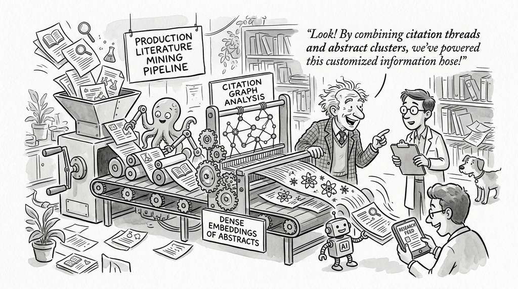
Semantic Scholar (developed by the Allen Institute for AI) uses a production literature mining pipeline that shares architectural principles with the one built here, combining citation graph analysis with dense embeddings of paper abstracts to power its "Research Feed" feature. The system harvests millions of papers, computes influence scores analogous to PageRank, clusters them into topical communities, and then recommends papers at the intersection of a researcher's reading history and trending structural holes in their field. The key architectural parallel is the staged pipeline: Semantic Scholar separates ingestion, graph construction, embedding, and recommendation into independently scalable services, exactly mirroring the six-stage checkpoint design of this section.
The Paper That Cited Itself Into Existence
In 2005, a group of researchers submitted a paper to a conference whose acceptance was partly predicted by a citation analysis algorithm. The paper's topic was citation analysis itself, and the authors included a self-citation in the references, creating a bootstrap loop: the algorithm used to evaluate the paper's importance counted the very paper it was evaluating. This edge case, known as a "citation fixed point," is surprisingly common in bibliometrics research and occasionally distorts PageRank scores in small citation graphs. The literature miner sidesteps this by filtering self-citations during graph construction, but if you remove that filter on a bibliometrics corpus, you will find that papers about citation metrics tend to appear more influential than they should be.
Lab: Mapping a Micro-Field with OpenAlex and NetworkX
Goal: Build a working literature miner for a 200-paper corpus and identify at least one structural hole in under 30 minutes.
Tools needed: Python 3.10+, requests, networkx, python-louvain (install via pip install python-louvain), matplotlib.
Procedure: (1) Query the OpenAlex API for 200 papers on a narrow topic of your choice (e.g., "federated learning healthcare"). (2) Parse the referenced_works field to build a directed citation graph with NetworkX. (3) Compute PageRank and run Louvain community detection on the undirected projection. (4) For every pair of communities with 5+ members, compute the ratio of actual cross-citations to expected cross-citations under a random null model. Flag pairs below 20% as structural holes.
What to vary: Try changing the Louvain resolution parameter from 0.5 to 2.0 in steps of 0.25 and observe how the number and size of detected communities change, and whether structural holes appear or vanish.
What to observe: At low resolution, communities merge and holes disappear; at high resolution, communities fragment and nearly every pair becomes a "hole." Record the resolution value that produces the highest modularity score; this is typically the most informative partition.