"The pipeline had four stages: estimate the effect, map the spillovers, simulate the counterfactual, and explain to the minister why all three disagreed. The last stage was the hardest."
A Policy Analyzer That Learned Diplomacy
A job training program lifts average earnings by \$3,200, and the minister calls it a success, until a deeper analysis reveals that workers under 30 gained \$8,500 while workers over 55 lost \$400 in seniority during training. The pipeline assembled here exists to surface exactly that kind of hidden distributional reality. It has four stages: (1) estimate heterogeneous treatment effects from observational data using EconML's causal forest, (2) compute network exposure features that capture treatment spillovers, (3) embed the estimated effects into an agent-based simulation for counterfactual projection, and (4) produce a distributional impact report with uncertainty quantification. The result is a system that answers the question every policymaker asks: "If we implement this policy, who benefits, who is harmed, and by how much?"
1. Pipeline Architecture
When India's demonetization policy withdrew 86% of circulating currency overnight in 2016, economists discovered months later that the program had devastated informal-sector workers while barely affecting salaried employees. That distributional blindness is not unusual; it is the default outcome when policy evaluation relies on a single aggregate number. The pipeline described here exists to prevent exactly that failure.
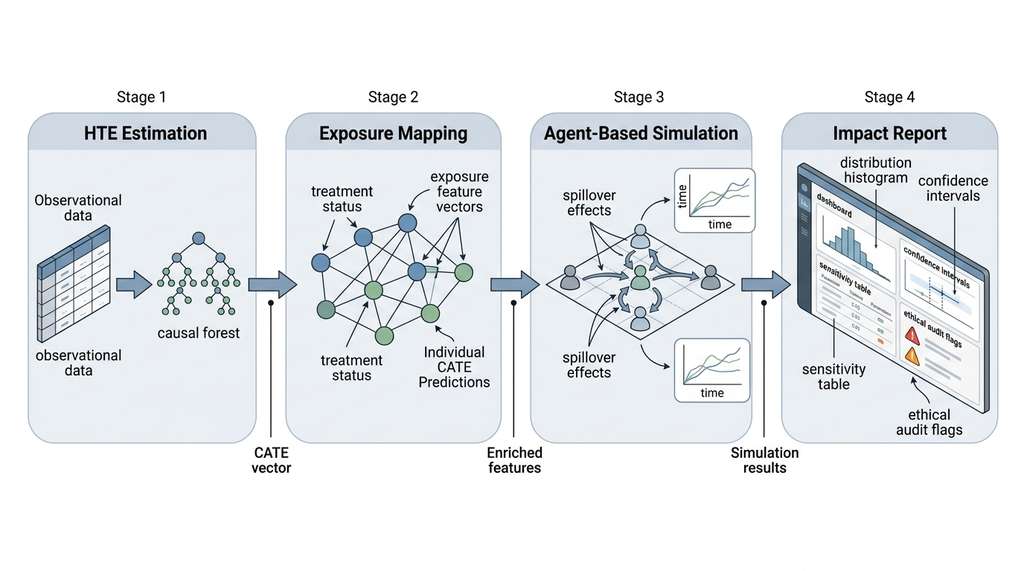
What. The Policy Impact Analyzer is a four-stage pipeline that combines statistical estimation with computational simulation. Stage 1 estimates conditional average treatment effects (CATEs) from historical data. Stage 2 enriches unit features with network exposure variables. Stage 3 feeds estimated CATEs into an agent-based model as behavioral parameters. Stage 4 aggregates agent-level outcomes into policy-relevant summaries with confidence intervals. The four-stage architecture is shown in Figure 52.16.
A conditional average treatment effect (CATE) measures the expected causal effect of a treatment on a specific subgroup defined by observed characteristics. For example, it captures the income boost from job training for workers aged 25 with a high school diploma. CATEs matter because policies rarely affect everyone equally; knowing that a program helps younger workers by \$5,000 but costs older workers \$400 in lost seniority is far more actionable than a single average. A causal forest partitions the covariate space into leaves where the treatment-control outcome difference is maximally heterogeneous, then estimates a local average effect within each leaf. Use CATEs (via causal forests or similar methods) when you suspect the treatment effect varies across subpopulations and you need to identify who benefits most. Use a simple average treatment effect (ATE) only when effect heterogeneity is not policy-relevant or when the sample is too small to support subgroup estimation.
Why. No single method provides a complete policy evaluation. Causal inference (Stage 1) estimates effects but cannot project them to novel contexts. Exposure mapping (Stage 2) accounts for interference but is static. Agent-based simulation (Stage 3) projects effects forward but requires calibration. By chaining these methods, we inherit each method's strength while using the others to compensate for its limitations.
How. The pipeline comprises composable Python classes, one per stage, connected by standardized intermediate representations. Any stage can be swapped (for example, replacing the causal forest with a double ML estimator, where "double" refers to the two-step nuisance-parameter estimation that first removes confounding from both the outcome and treatment before estimating the causal effect) without modifying the rest of the pipeline. Figure 52.4.1 illustrates the four-stage Policy Impact Analyzer pipeline architecture.
When. Use this pipeline when evaluating a policy intervention that (1) has some historical or quasi-experimental data from which treatment effects can be estimated, (2) operates in a networked setting where spillovers matter, and (3) requires projection to a new context (different population, different scale, different complementary policies). If any of these conditions is missing, the individual components from Sections 52.1 through 52.3 may be used independently. In short: Estimate who gains, map who spills over, simulate what happens next, and only then decide whether the policy is worth funding.
The most common criticism of agent-based models is that their behavioral rules are arbitrary. The most common criticism of causal inference is that it cannot extrapolate. This pipeline addresses both: the causal forest provides empirically grounded, heterogeneous effect estimates that become the agents' behavioral parameters. The simulation then extrapolates these effects to new settings, new population compositions, and new policy combinations. The estimates constrain the simulation; the simulation extends the estimates. Neither alone provides what the combination delivers.
Mental Model
Think of the estimation-then-simulation pipeline like a weather forecast. A meteorologist first measures current conditions at hundreds of weather stations (analogous to estimating CATEs from observed data: precise, local, grounded in measurement). Those readings then initialize a physics-based atmospheric simulation that projects the weather forward in time and to locations between stations (analogous to the agent-based model extrapolating effects to new populations and future periods). The measurements alone cannot predict tomorrow's weather, and the simulation alone would drift without real data to anchor it. The forecast's value comes from grounding the simulation in measurement, exactly as this pipeline grounds agent behavior in causal estimates.
2. Stage 1: Heterogeneous Treatment Effect Estimation
We use EconML, a Python library from Microsoft Research for causal machine learning, specifically its CausalForestDML, which combines the double machine learning framework of Chernozhukov et al. (2018) with the causal forest of Athey, Tibshirani, and Wager (2019). The estimator produces individual-level treatment effect predictions \(\hat{\tau}(X_i)\) that vary with observed covariates, revealing which subgroups benefit most from the policy.
Common Misconception
A frequent mistake is treating the average treatment effect (ATE) as if it applies uniformly to every individual, then concluding that a positive ATE means the policy helps everyone. In reality, a positive ATE of \$3,000 can mask a distribution where half the population gains \$8,000 and the other half loses \$2,000. Always inspect the full CATE distribution (especially the fraction with negative effects) before recommending a policy, because the average can hide substantial harm to specific subgroups.
import numpy as np
import pandas as pd
from sklearn.ensemble import GradientBoostingRegressor, GradientBoostingClassifier
from econml.dml import CausalForestDML
from dataclasses import dataclass, field
from typing import Optional
import networkx as nx


@dataclass
class HTEResults:
    """Results from heterogeneous treatment effect estimation."""
    cate_predictions: np.ndarray
    ate: float
    ate_ci: tuple
    feature_importances: dict
    model: object


class HTEEstimator:
    """
    Stage 1: Estimate heterogeneous treatment effects
    using EconML's CausalForestDML.

    This stage takes observational data with a binary treatment,
    outcome, and covariates, and produces individual-level
    treatment effect predictions.
    """

    def __init__(
        self,
        n_estimators: int = 200,
        min_samples_leaf: int = 10,
        max_depth: int = None,
        random_state: int = 42,
    ):
        self.model = CausalForestDML(
            model_y=GradientBoostingRegressor(
                n_estimators=100, max_depth=5, random_state=random_state
            ),
            model_t=GradientBoostingClassifier(
                n_estimators=100, max_depth=5, random_state=random_state
            ),
            n_estimators=n_estimators,
            min_samples_leaf=min_samples_leaf,
            max_depth=max_depth,
            random_state=random_state,
        )

    def fit(
        self,
        data: pd.DataFrame,
        outcome_col: str,
        treatment_col: str,
        covariate_cols: list,
        effect_modifier_cols: list = None,
    ) -> HTEResults:
        """
        Fit the causal forest and estimate CATEs.

        Parameters
        ----------
        data : observational dataset
        outcome_col : name of the outcome variable
        treatment_col : name of the binary treatment variable
        covariate_cols : confounders to control for
        effect_modifier_cols : variables that modify the treatment
            effect (used as X in EconML). If None, uses covariate_cols.

        Returns
        -------
        HTEResults with CATE predictions and diagnostics
        """
        Y = data[outcome_col].values
        T = data[treatment_col].values
        W = data[covariate_cols].values  # Confounders

        if effect_modifier_cols is None:
            effect_modifier_cols = covariate_cols
        X = data[effect_modifier_cols].values  # Effect modifiers

        # Fit the causal forest
        self.model.fit(Y, T, X=X, W=W)

        # Predict individual treatment effects
        cate_predictions = self.model.effect(X).flatten()

        # Average treatment effect with confidence interval
        ate_inference = self.model.ate_inference(X=X)
        ate = ate_inference.point_estimate
        ate_ci = (ate_inference.conf_int()[0][0], ate_inference.conf_int()[1][0])

        # Feature importances for interpretability
        importances = dict(zip(
            effect_modifier_cols,
            self.model.feature_importances_
        ))

        return HTEResults(
            cate_predictions=cate_predictions,
            ate=float(ate),
            ate_ci=(float(ate_ci[0]), float(ate_ci[1])),
            feature_importances=importances,
            model=self.model,
        )


# Generate synthetic observational data for a job training program
np.random.seed(42)
n = 3000

age = np.random.uniform(22, 60, n)
education = np.random.choice([10, 12, 14, 16, 18], n, p=[0.1, 0.3, 0.25, 0.25, 0.1])
prior_income = 20000 + 2000 * education + 500 * age + np.random.normal(0, 5000, n)
prior_income = np.maximum(prior_income, 10000)

# Treatment assignment (non-random: depends on covariates)
# Propensity: the probability that a unit receives treatment,
# given its observed covariates
propensity = 1 / (1 + np.exp(
    -(0.05 * (age - 40) - 0.3 * (education - 14) + 0.00002 * (prior_income - 50000))
))
treatment = np.random.binomial(1, propensity)

# Heterogeneous treatment effect: larger for younger, less educated
true_cate = 5000 - 80 * age + 200 * (16 - education)
true_cate = np.maximum(true_cate, -1000)  # Floor

# Outcome: post-program income
post_income = (
    prior_income + 1000
    + true_cate * treatment
    + np.random.normal(0, 3000, n)
)

obs_data = pd.DataFrame({
    "age": age,
    "education": education,
    "prior_income": prior_income,
    "treatment": treatment,
    "post_income": post_income,
})

# Fit the causal forest
hte_estimator = HTEEstimator(n_estimators=200)
hte_results = hte_estimator.fit(
    obs_data,
    outcome_col="post_income",
    treatment_col="treatment",
    covariate_cols=["age", "education", "prior_income"],
    effect_modifier_cols=["age", "education"],
)

print(f"ATE: ${hte_results.ate:,.0f}")
print(f"95% CI: [${hte_results.ate_ci[0]:,.0f}, ${hte_results.ate_ci[1]:,.0f}]")
print(f"\nFeature importances:")
for feat, imp in sorted(
    hte_results.feature_importances.items(),
    key=lambda x: x[1], reverse=True,
):
    print(f"  {feat}: {imp:.4f}")

# CATE distribution
print(f"\nCATE distribution:")
print(f"  Mean: ${np.mean(hte_results.cate_predictions):,.0f}")
print(f"  Std:  ${np.std(hte_results.cate_predictions):,.0f}")
print(f"  Min:  ${np.min(hte_results.cate_predictions):,.0f}")
print(f" Max: ${np.max(hte_results.cate_predictions):,.0f}")With individual treatment effect estimates in hand, the next question is whether those estimates hold when units influence one another; in most social settings, they do not, because a treated individual's outcome spills over to untreated neighbors.
3. Stage 2: Exposure Mapping for Network Interference
The causal forest in Stage 1 assumes the stable unit treatment value assumption (SUTVA): each unit's outcome depends only on its own treatment status. In social systems, this assumption typically fails. When 40% of a worker's neighbors also receive job training, that worker's outcome reflects not just her own treatment but the changed competitive landscape around her, so the individual-level CATE estimate is biased by construction unless exposure is modeled explicitly. Stage 2 enriches the feature set with network exposure variables. These variables capture the fraction of each unit's neighbors who are treated, the average CATE among neighbors, and centrality-based measures of network position.
Checkpoint
So far: Stage 1 assumed each unit's outcome depends only on its own treatment (SUTVA), but social settings violate that assumption because treated neighbors change the competitive landscape; Stage 2 now quantifies that violation by computing exposure features (neighbor treatment fraction, neighbor mean CATE, centrality) for every unit in the network.
@dataclass
class ExposureFeatures:
    """Network exposure features for each unit."""
    features: pd.DataFrame
    network_stats: dict


class ExposureMapper:
    """
    Stage 2: Compute network exposure features that capture
    treatment spillovers for interference-aware estimation.
    """

    def __init__(self, graph: nx.Graph):
        self.graph = graph
        self._centralities = None

    def compute_exposure(
        self,
        treatment: np.ndarray,
        cate_predictions: np.ndarray,
        node_ids: list,
    ) -> ExposureFeatures:
        """
        Compute exposure features for each unit based on
        network position and neighbors' treatment status.

        Parameters
        ----------
        treatment : binary treatment vector
        cate_predictions : predicted CATEs from Stage 1
        node_ids : identifiers mapping data rows to graph nodes

        Returns
        -------
        ExposureFeatures with enriched feature set
        """
        treatment_map = dict(zip(node_ids, treatment))
        cate_map = dict(zip(node_ids, cate_predictions))

        # Compute centrality measures (cached)
        if self._centralities is None:
            self._centralities = {
                "pagerank": nx.pagerank(self.graph),
                "betweenness": nx.betweenness_centrality(self.graph),
                "clustering": nx.clustering(self.graph),
            }

        exposure_rows = []
        for node_id in node_ids:
            if node_id not in self.graph:
                exposure_rows.append({
                    "node_id": node_id,
                    "neighbor_treatment_frac": 0.0,
                    "neighbor_mean_cate": 0.0,
                    "neighbor_count": 0,
                    "treated_neighbor_count": 0,
                    "pagerank": 0.0,
                    "betweenness": 0.0,
                    "clustering": 0.0,
                    "two_hop_exposure": 0.0,
                })
                continue

            neighbors = list(self.graph.neighbors(node_id))
            n_neighbors = len(neighbors)

            if n_neighbors == 0:
                exposure_rows.append({
                    "node_id": node_id,
                    "neighbor_treatment_frac": 0.0,
                    "neighbor_mean_cate": 0.0,
                    "neighbor_count": 0,
                    "treated_neighbor_count": 0,
                    "pagerank": self._centralities["pagerank"].get(node_id, 0),
                    "betweenness": self._centralities["betweenness"].get(node_id, 0),
                    "clustering": self._centralities["clustering"].get(node_id, 0),
                    "two_hop_exposure": 0.0,
                })
                continue

            # 1-hop exposure: fraction of neighbors treated
            treated_neighbors = sum(
                treatment_map.get(n, 0) for n in neighbors
            )
            neighbor_treatment_frac = treated_neighbors / n_neighbors

            # Mean predicted CATE among neighbors
            neighbor_cates = [
                cate_map.get(n, 0) for n in neighbors
            ]
            neighbor_mean_cate = np.mean(neighbor_cates)

            # 2-hop exposure: fraction of 2-hop neighbors treated
            two_hop = set()
            for n1 in neighbors:
                if n1 in self.graph:
                    for n2 in self.graph.neighbors(n1):
                        if n2 != node_id and n2 not in neighbors:
                            two_hop.add(n2)
            two_hop_treated = sum(
                treatment_map.get(n, 0) for n in two_hop
            )
            two_hop_exposure = (
                two_hop_treated / len(two_hop) if two_hop else 0.0
            )

            exposure_rows.append({
                "node_id": node_id,
                "neighbor_treatment_frac": neighbor_treatment_frac,
                "neighbor_mean_cate": neighbor_mean_cate,
                "neighbor_count": n_neighbors,
                "treated_neighbor_count": treated_neighbors,
                "pagerank": self._centralities["pagerank"].get(node_id, 0),
                "betweenness": self._centralities["betweenness"].get(node_id, 0),
                "clustering": self._centralities["clustering"].get(node_id, 0),
                "two_hop_exposure": two_hop_exposure,
            })

        features_df = pd.DataFrame(exposure_rows)

        # Network-level summary statistics
        network_stats = {
            "mean_exposure": features_df["neighbor_treatment_frac"].mean(),
            "exposure_std": features_df["neighbor_treatment_frac"].std(),
            "mean_two_hop": features_df["two_hop_exposure"].mean(),
            "treatment_clustering": self._treatment_clustering(
                treatment_map
            ),
        }

        return ExposureFeatures(
            features=features_df, network_stats=network_stats
        )

    def _treatment_clustering(self, treatment_map: dict) -> float:
        """
        Measure how clustered the treatment is in the network.
        High values indicate treated units are neighbors of
        treated units (geographic/social clustering of policy).
        """
        edges_both_treated = 0
        edges_any_treated = 0
        for u, v in self.graph.edges():
            t_u = treatment_map.get(u, 0)
            t_v = treatment_map.get(v, 0)
            if t_u or t_v:
                edges_any_treated += 1
                if t_u and t_v:
                    edges_both_treated += 1
        if edges_any_treated == 0:
            return 0.0
        return edges_both_treated / edges_any_treated


# Create a social network for the 3000 individuals
# Watts-Strogatz graph: a network model that starts from a ring
# lattice and rewires each edge with probability p, producing
# realistic "small-world" structure (high clustering, short paths)
social_graph = nx.watts_strogatz_graph(n, 8, 0.15, seed=42)
node_ids = list(range(n))

# Compute exposure features
mapper = ExposureMapper(social_graph)
exposure = mapper.compute_exposure(
    treatment=treatment,
    cate_predictions=hte_results.cate_predictions,
    node_ids=node_ids,
)

print("Exposure feature statistics:")
print(exposure.features.describe().round(4))
print(f"\nNetwork-level stats: {exposure.network_stats}")Now that each unit carries both an estimated treatment effect and a set of exposure features describing its network context, the pipeline can move from static estimation to dynamic projection by embedding these parameters into a simulation.
4. Stage 3: Agent-Based Counterfactual Simulation
Stage 3 embeds the estimated CATEs from Stage 1 and the exposure features from Stage 2 into an agent-based simulation that projects policy effects forward. Each simulated agent's response to treatment is parameterized by the CATE estimated for units with similar covariates, and spillover effects are mediated by the network structure. The simulation uses Mesa, a Python framework for agent-based modeling that provides scheduling, data collection, and network-aware agent interaction out of the box.
import mesa


class PolicyAgent(mesa.Agent):
    """
    An agent whose treatment response is parameterized
    by empirically estimated CATEs and network exposure.
    """

    def __init__(
        self,
        model,
        covariates: dict,
        estimated_cate: float,
        network_exposure: float,
        is_treated: bool = False,
    ):
        super().__init__(model)
        self.covariates = covariates
        self.estimated_cate = estimated_cate
        self.network_exposure = network_exposure
        self.is_treated = is_treated
        self.outcome = covariates.get("baseline_outcome", 0)
        self.cumulative_effect = 0.0

    def step(self):
        """
        Update outcome based on treatment, own CATE,
        and neighborhood spillover effects.
        """
        if self.is_treated:
            # Direct treatment effect (from causal forest)
            direct = self.estimated_cate
        else:
            direct = 0.0

        # Spillover effect: proportional to network exposure
        # and the average CATE among treated neighbors
        spillover_rate = self.model.spillover_coefficient
        spillover = (
            spillover_rate * self.network_exposure
            * self.estimated_cate
        )

        # Time-varying effect: ramp up over first 12 periods
        # then stabilize (captures program maturation)
        step_num = self.model.schedule_step
        ramp = min(1.0, step_num / 12.0)

        period_effect = ramp * (direct + spillover)
        self.cumulative_effect += period_effect
        self.outcome = (
            self.covariates.get("baseline_outcome", 0)
            + self.cumulative_effect
            + np.random.normal(0, 500)  # Idiosyncratic shock
        )


class PolicySimulation(mesa.Model):
    """
    Stage 3: Agent-based policy simulation parameterized
    by empirically estimated treatment effects.
    """

    def __init__(
        self,
        agent_data: pd.DataFrame,
        graph: nx.Graph,
        spillover_coefficient: float = 0.3,
        seed: int = 42,
    ):
        """
        Parameters
        ----------
        agent_data : DataFrame with columns 'node_id', 'covariates',
            'estimated_cate', 'network_exposure', 'is_treated'
        graph : social network
        spillover_coefficient : strength of network spillovers
        """
        super().__init__(seed=seed)
        self.graph = graph
        self.spillover_coefficient = spillover_coefficient
        self.schedule_step = 0

        # Create agents from data
        for _, row in agent_data.iterrows():
            PolicyAgent(
                self,
                covariates=row.get("covariates", {}),
                estimated_cate=row["estimated_cate"],
                network_exposure=row["network_exposure"],
                is_treated=row["is_treated"],
            )

        self.datacollector = mesa.DataCollector(
            model_reporters={
                "mean_outcome": lambda m: np.mean([
                    a.outcome for a in m.agents
                ]),
                "treated_mean_outcome": lambda m: np.mean([
                    a.outcome for a in m.agents if a.is_treated
                ] or [0]),
                "control_mean_outcome": lambda m: np.mean([
                    a.outcome for a in m.agents if not a.is_treated
                ] or [0]),
                "outcome_gini": lambda m: self._gini([
                    a.outcome for a in m.agents
                ]),
                "mean_cumulative_effect": lambda m: np.mean([
                    a.cumulative_effect for a in m.agents
                ]),
            },
            agent_reporters={
                "outcome": "outcome",
                "cumulative_effect": "cumulative_effect",
                "is_treated": "is_treated",
            },
        )

    def step(self):
        self.schedule_step += 1
        self.agents.shuffle_do("step")
        self.datacollector.collect(self)

    @staticmethod
    def _gini(values):
        sorted_vals = sorted([v for v in values if v > 0])
        n = len(sorted_vals)
        if n < 2:
            return 0.0
        cumulative = np.cumsum(sorted_vals)
        return (
            (2 * np.sum((np.arange(1, n + 1) * sorted_vals)))
            / (n * cumulative[-1])
            - (n + 1) / n
        )


# Prepare agent data for simulation
agent_df = pd.DataFrame({
    "node_id": node_ids,
    "estimated_cate": hte_results.cate_predictions,
    "network_exposure": exposure.features["neighbor_treatment_frac"].values,
    "is_treated": treatment.astype(bool),
    "covariates": [
        {
            "baseline_outcome": obs_data.loc[i, "prior_income"],
            "age": obs_data.loc[i, "age"],
            "education": obs_data.loc[i, "education"],
        }
        for i in range(n)
    ],
})

# Run simulation for 24 periods (e.g., months)
sim = PolicySimulation(
    agent_df, social_graph,
    spillover_coefficient=0.3, seed=42,
)
for _ in range(24):
    sim.step()

sim_results = sim.datacollector.get_model_dataframe()
print("\nSimulation results (24-period projection):")
print(sim_results.tail(5).to_string())The simulation generates rich, agent-level outcome trajectories, but raw trajectories are not yet actionable for a policymaker; Stage 4 wraps the preceding three stages into a single callable pipeline that aggregates results into distributional summaries, confidence intervals, and sensitivity checks.
5. Stage 4: The Complete Pipeline
The PolicyImpactAnalyzer class orchestrates all four stages into a single callable pipeline. It accepts observational data, a network, and a policy specification, and produces a comprehensive impact report with point estimates, confidence intervals, distributional breakdowns, and sensitivity checks. The report includes the Gini coefficient (a measure of inequality ranging from 0 for perfect equality to 1 for maximal inequality) of outcomes to flag policies that concentrate gains in a narrow subpopulation.
@dataclass
class PolicyImpactReport:
    """Complete output from the Policy Impact Analyzer."""
    ate: float
    ate_ci: tuple
    cate_distribution: dict
    distributional_effects: pd.DataFrame
    simulation_trajectory: pd.DataFrame
    network_spillover_estimate: float
    sensitivity_results: dict
    feature_importances: dict


class PolicyImpactAnalyzer:
    """
    End-to-end policy evaluation pipeline combining:
    1. Heterogeneous treatment effect estimation (EconML)
    2. Network exposure mapping (NetworkX)
    3. Agent-based counterfactual simulation (Mesa)
    4. Distributional impact reporting

    Integrates with the Discovery Workbench as a
    domain-specific analysis module.
    """

    def __init__(
        self,
        n_estimators: int = 200,
        spillover_coefficient: float = 0.3,
        simulation_periods: int = 24,
        n_replications: int = 5,
        random_state: int = 42,
    ):
        self.hte_estimator = HTEEstimator(
            n_estimators=n_estimators, random_state=random_state
        )
        self.spillover_coefficient = spillover_coefficient
        self.simulation_periods = simulation_periods
        self.n_replications = n_replications
        self.random_state = random_state

    def analyze(
        self,
        data: pd.DataFrame,
        graph: nx.Graph,
        outcome_col: str,
        treatment_col: str,
        covariate_cols: list,
        effect_modifier_cols: list = None,
        group_col: str = None,
    ) -> PolicyImpactReport:
        """
        Run the complete policy impact analysis.

        Parameters
        ----------
        data : observational dataset
        graph : social/economic network
        outcome_col : outcome variable
        treatment_col : binary treatment indicator
        covariate_cols : confounders to control for
        effect_modifier_cols : variables that modify treatment effect
        group_col : column for distributional analysis subgroups

        Returns
        -------
        PolicyImpactReport with all results
        """
        # Stage 1: Estimate heterogeneous treatment effects
        hte = self.hte_estimator.fit(
            data, outcome_col, treatment_col,
            covariate_cols, effect_modifier_cols,
        )

        # Stage 2: Compute network exposure
        node_ids = list(range(len(data)))
        mapper = ExposureMapper(graph)
        exposure = mapper.compute_exposure(
            treatment=data[treatment_col].values,
            cate_predictions=hte.cate_predictions,
            node_ids=node_ids,
        )

        # Stage 3: Run agent-based simulation with replications
        all_trajectories = []
        for rep in range(self.n_replications):
            agent_df = pd.DataFrame({
                "node_id": node_ids,
                "estimated_cate": hte.cate_predictions,
                "network_exposure": (
                    exposure.features["neighbor_treatment_frac"].values
                ),
                "is_treated": data[treatment_col].astype(bool).values,
                "covariates": [
                    {
                        "baseline_outcome": data.iloc[i][outcome_col],
                        **{c: data.iloc[i][c] for c in covariate_cols},
                    }
                    for i in range(len(data))
                ],
            })

            sim = PolicySimulation(
                agent_df, graph,
                spillover_coefficient=self.spillover_coefficient,
                seed=self.random_state + rep,
            )
            for _ in range(self.simulation_periods):
                sim.step()

            traj = sim.datacollector.get_model_dataframe()
            traj["replication"] = rep
            all_trajectories.append(traj)

        trajectories_df = pd.concat(all_trajectories)

        # Stage 4: Compile results
        # Distributional effects by subgroup
        dist_effects = self._distributional_analysis(
            data, hte.cate_predictions, group_col
        )

        # CATE distribution summary
        cate_dist = {
            "mean": float(np.mean(hte.cate_predictions)),
            "std": float(np.std(hte.cate_predictions)),
            "median": float(np.median(hte.cate_predictions)),
            "q10": float(np.percentile(hte.cate_predictions, 10)),
            "q25": float(np.percentile(hte.cate_predictions, 25)),
            "q75": float(np.percentile(hte.cate_predictions, 75)),
            "q90": float(np.percentile(hte.cate_predictions, 90)),
            "fraction_positive": float(
                np.mean(hte.cate_predictions > 0)
            ),
            "fraction_negative": float(
                np.mean(hte.cate_predictions < 0)
            ),
        }

        # Sensitivity: vary spillover coefficient
        sensitivity = self._sensitivity_analysis(
            hte.cate_predictions, exposure.features, data,
            outcome_col, covariate_cols,
        )

        # Network spillover estimate
        spillover_est = (
            self.spillover_coefficient
            * exposure.network_stats["mean_exposure"]
            * np.mean(hte.cate_predictions)
        )

        return PolicyImpactReport(
            ate=hte.ate,
            ate_ci=hte.ate_ci,
            cate_distribution=cate_dist,
            distributional_effects=dist_effects,
            simulation_trajectory=trajectories_df,
            network_spillover_estimate=spillover_est,
            sensitivity_results=sensitivity,
            feature_importances=hte.feature_importances,
        )

    def _distributional_analysis(
        self,
        data: pd.DataFrame,
        cate_predictions: np.ndarray,
        group_col: str = None,
    ) -> pd.DataFrame:
        """Analyze treatment effects by subgroup."""
        df = data.copy()
        df["predicted_cate"] = cate_predictions

        if group_col and group_col in df.columns:
            groups = df.groupby(group_col)["predicted_cate"].agg(
                ["mean", "std", "count",
                 lambda x: np.mean(x > 0)]
            )
            groups.columns = [
                "mean_cate", "std_cate", "n",
                "fraction_positive",
            ]
            return groups.reset_index()

        # Default: quintile analysis
        df["cate_quintile"] = pd.qcut(
            cate_predictions, 5,
            labels=["Q1 (lowest)", "Q2", "Q3", "Q4", "Q5 (highest)"]
        )
        return df.groupby("cate_quintile").agg(
            mean_cate=("predicted_cate", "mean"),
            n=("predicted_cate", "count"),
        ).reset_index()

    def _sensitivity_analysis(
        self,
        cate_predictions: np.ndarray,
        exposure_features: pd.DataFrame,
        data: pd.DataFrame,
        outcome_col: str,
        covariate_cols: list,
    ) -> dict:
        """
        Sensitivity analysis: how do results change under
        different spillover assumptions?
        """
        spillover_values = [0.0, 0.1, 0.3, 0.5, 0.7]
        results = {}
        mean_exposure = exposure_features[
            "neighbor_treatment_frac"
        ].mean()

        for spill in spillover_values:
            total_effect = np.mean(cate_predictions) * (
                1 + spill * mean_exposure
            )
            results[f"spillover_{spill}"] = {
                "spillover_coefficient": spill,
                "total_effect": total_effect,
                "amplification_factor": 1 + spill * mean_exposure,
            }

        return results


# Run the complete pipeline
analyzer = PolicyImpactAnalyzer(
    n_estimators=200,
    spillover_coefficient=0.3,
    simulation_periods=24,
    n_replications=3,
)

# Add an education group column for distributional analysis
obs_data["education_group"] = pd.cut(
    obs_data["education"],
    bins=[0, 12, 14, 20],
    labels=["High School", "Some College", "College+"],
)

report = analyzer.analyze(
    data=obs_data,
    graph=social_graph,
    outcome_col="post_income",
    treatment_col="treatment",
    covariate_cols=["age", "education", "prior_income"],
    effect_modifier_cols=["age", "education"],
    group_col="education_group",
)

print("=" * 60)
print("POLICY IMPACT REPORT: Job Training Program")
print("=" * 60)
print(f"\nAverage Treatment Effect: ${report.ate:,.0f}")
print(f"95% CI: [${report.ate_ci[0]:,.0f}, ${report.ate_ci[1]:,.0f}]")
print(f"\nCATE Distribution:")
for key, val in report.cate_distribution.items():
    if isinstance(val, float):
        if "fraction" in key:
            print(f"  {key}: {val:.1%}")
        else:
            print(f"  {key}: ${val:,.0f}")
print(f"\nNetwork Spillover Estimate: ${report.network_spillover_estimate:,.0f}")
print(f"\nDistributional Effects by Education:")
print(report.distributional_effects.to_string(index=False))
print(f"\nFeature Importances:")
for feat, imp in sorted(
    report.feature_importances.items(),
    key=lambda x: x[1], reverse=True,
):
    print(f"  {feat}: {imp:.4f}")
print(f"\nSensitivity to Spillover Coefficient:")
for key, val in report.sensitivity_results.items():
    print(
        f"  {val['spillover_coefficient']:.1f}: "
        f"total effect = ${val['total_effect']:,.0f} "
        f"(amplification: {val['amplification_factor']:.2f}x)"
)analyze method chains HTE estimation, exposure mapping, replicated ABM simulation, and distributional reporting into a single call that returns a PolicyImpactReport with CATE quantiles, subgroup breakdowns, and spillover sensitivity.A state workforce agency deploys the Policy Impact Analyzer to evaluate a \$50 million job training program. The pipeline ingests administrative data on 150,000 workers (employment histories, demographics, training participation) and a commuting-zone network connecting 200 labor markets. Stage 1 reveals that the program increases annual earnings by \$3,200 on average, but CATEs range from \$8,500 for workers under 30 without college degrees to negative \$400 for workers over 55 (who lose seniority during training). Stage 2 shows that treatment is clustered in urban areas, creating exposure of 0.45 in cities versus 0.08 in rural zones. Stage 3's simulation projects that with the current spillover coefficient (0.3), the program generates \$180 million in additional earnings over 3 years, but 60% of gains concentrate in 20% of communities. The agency uses the distributional breakdown to redesign the program: expanding eligibility for younger workers, adding wage insurance for older workers during training, and targeting rural communities for additional outreach.
Research Frontier
Athey et al. (2024) introduced the Causal Forest with Approximate Residual Balancing (CF-ARB), which integrates balancing weights directly into the forest splitting criterion to reduce bias from strong confounding in observational studies. Their method, implemented in the updated grf R package (version 2.4+) and being ported to EconML, achieves sharper CATE confidence intervals and better calibration under near-violations of overlap (positivity). Separately, Viviano et al. (2024) proposed "causal forests under interference" that jointly estimate direct and spillover effects within a single forest, eliminating the need for the two-stage estimation-then-exposure-mapping approach used in this section. These advances push toward end-to-end pipelines where effect heterogeneity and network interference are handled in a unified estimation step rather than sequentially.
6. Discovery Workbench Integration
The Policy Impact Analyzer integrates into the Discovery Workbench as a domain-specific analysis module, connecting to the broader ecosystem of discovery tools introduced throughout this book.
class SocialEconomicDiscoveryModule:
    """
    Discovery Workbench integration for social and economic
    systems analysis. Orchestrates network analysis (52.1),
    causal inference (52.2), and policy simulation (52.3)
    into a unified discovery pipeline.

    Connects to:
    - Knowledge Graph (Ch 38): policy ontology and evidence linking
    - Experiment Registry (Ch 47): logging analysis provenance
    - Causal Discovery (Ch 31): structural model specification
    - Responsible AI (Ch 57): ethical constraint checking
    """

    def __init__(self, config: dict = None):
        self.config = config or {}
        self.analyzer = PolicyImpactAnalyzer(
            n_estimators=self.config.get("n_estimators", 200),
            spillover_coefficient=self.config.get("spillover", 0.3),
            simulation_periods=self.config.get("sim_periods", 24),
            n_replications=self.config.get("n_replications", 5),
        )
        self.results_history = []

    def run_analysis(
        self,
        data: pd.DataFrame,
        graph: nx.Graph,
        policy_name: str,
        outcome_col: str,
        treatment_col: str,
        covariate_cols: list,
        **kwargs,
    ) -> PolicyImpactReport:
        """
        Run a named policy analysis and log it to the
        experiment registry.
        """
        report = self.analyzer.analyze(
            data=data,
            graph=graph,
            outcome_col=outcome_col,
            treatment_col=treatment_col,
            covariate_cols=covariate_cols,
            **kwargs,
        )

        # Log to experiment registry
        entry = {
            "policy_name": policy_name,
            "n_observations": len(data),
            "n_network_nodes": graph.number_of_nodes(),
            "ate": report.ate,
            "ate_ci": report.ate_ci,
            "fraction_positive_cate": (
                report.cate_distribution["fraction_positive"]
            ),
            "spillover_estimate": report.network_spillover_estimate,
        }
        self.results_history.append(entry)

        return report

    def compare_policies(
        self, reports: dict
    ) -> pd.DataFrame:
        """
        Compare multiple policy analyses side by side.

        Parameters
        ----------
        reports : dict mapping policy names to PolicyImpactReports

        Returns
        -------
        DataFrame comparing key metrics across policies
        """
        comparison = []
        for name, report in reports.items():
            comparison.append({
                "policy": name,
                "ate": report.ate,
                "ate_ci_lower": report.ate_ci[0],
                "ate_ci_upper": report.ate_ci[1],
                "fraction_benefiting": (
                    report.cate_distribution["fraction_positive"]
                ),
                "cate_q10": report.cate_distribution["q10"],
                "cate_q90": report.cate_distribution["q90"],
                "spillover": report.network_spillover_estimate,
            })

        return pd.DataFrame(comparison).sort_values(
            "ate", ascending=False
        )

    def ethical_audit(self, report: PolicyImpactReport) -> dict:
        """
        Check policy evaluation against ethical constraints.

        Flags:
        - Policies where >20% of the population is harmed
        - Policies with highly unequal distributional effects
        - Results sensitive to spillover specification
        """
        flags = []

        frac_neg = report.cate_distribution["fraction_negative"]
        if frac_neg > 0.20:
            flags.append({
                "type": "harm",
                "severity": "high" if frac_neg > 0.40 else "medium",
                "message": (
                    f"{frac_neg:.0%} of the population is predicted "
                    f"to be harmed by this policy."
                ),
            })

        # Check distributional inequality
        q90_q10_ratio = abs(
            report.cate_distribution["q90"]
            / (report.cate_distribution["q10"] or 1)
        )
        if q90_q10_ratio > 5:
            flags.append({
                "type": "inequality",
                "severity": "medium",
                "message": (
                    f"Treatment effect inequality is high: "
                    f"Q90/Q10 ratio = {q90_q10_ratio:.1f}."
                ),
            })

        # Check sensitivity to spillover specification
        spill_vals = list(report.sensitivity_results.values())
        effects = [v["total_effect"] for v in spill_vals]
        if max(effects) > 2 * min(effects):
            flags.append({
                "type": "sensitivity",
                "severity": "medium",
                "message": (
                    "Results are sensitive to spillover specification. "
                    "Total effect ranges from "
                    f"${min(effects):,.0f} to ${max(effects):,.0f}."
                ),
            })

        return {
            "flags": flags,
            "n_flags": len(flags),
            "recommendation": (
                "Proceed with caution" if flags
                else "No ethical concerns flagged"
            ),
        }


# Demonstrate the complete workflow
workbench = SocialEconomicDiscoveryModule(config={
    "n_estimators": 200,
    "spillover": 0.3,
    "sim_periods": 24,
    "n_replications": 3,
})

# Run and audit
audit = workbench.ethical_audit(report)
print("\nEthical Audit Results:")
print(f"  Flags: {audit['n_flags']}")
for flag in audit["flags"]:
    print(f"  [{flag['severity'].upper()}] {flag['type']}: {flag['message']}")
print(f" Recommendation: {audit['recommendation']}")run_analysis method logs provenance, compare_policies ranks alternatives by ATE and distributional spread, and ethical_audit flags policies that harm more than 20% of the population or show high sensitivity to spillover assumptions.The complete Stage 1 estimation (the HTEEstimator class, roughly 60 lines) condenses to about 15 lines using EconML and DoWhy directly:
from econml.dml import CausalForestDML
from sklearn.ensemble import GradientBoostingRegressor as GBR
from sklearn.ensemble import GradientBoostingClassifier as GBC

# Fit causal forest with Double ML
cf = CausalForestDML(model_y=GBR(), model_t=GBC(), n_estimators=200)
cf.fit(Y=df["income"], T=df["treatment"],
       X=df[["age", "education"]], W=df[["prior_income"]])

# Individual treatment effects
cates = cf.effect(df[["age", "education"]])

# ATE with confidence interval
ate_inf = cf.ate_inference(X=df[["age", "education"]])
print(f"ATE: {ate_inf.point_estimate:.0f}")
print(f"CI: {ate_inf.conf_int()}")

# Feature importances
print(f"Importances: {cf.feature_importances_}")EconML handles the cross-fitting (a procedure that splits data into folds, estimates nuisance parameters on one fold, and predicts treatment effects on the held-out fold to avoid overfitting bias), nuisance estimation, forest construction, and inference internally. The 200+ lines of pipeline code above exist to show how the estimation connects to exposure mapping, simulation, and ethical auditing, which are not part of EconML's scope.
Try It: Mini Policy Analyzer on Synthetic Data
Build a simplified version of the Policy Impact Analyzer on your laptop using only Python standard libraries plus numpy, pandas, scikit-learn, econml, networkx, and matplotlib. Follow these steps:
1. Generate synthetic data. Create a DataFrame of 1,000 individuals with age (uniform 20 to 60), years of education (categorical: 10, 12, 14, 16), and a binary treatment assigned with probability depending on age (younger workers more likely treated). Define a heterogeneous true effect: true_cate = 3000 - 60 * age, so younger workers benefit more. Simulate the outcome as baseline income plus true_cate * treatment plus Gaussian noise.
2. Estimate CATEs with EconML. Fit a CausalForestDML with model_y=GradientBoostingRegressor() and model_t=GradientBoostingClassifier(). Use age and education as effect modifiers (X) and all covariates as confounders (W). Extract per-individual CATE predictions and print the ATE with its 95% confidence interval.
3. Build a network and compute exposure. Generate a Watts-Strogatz graph (a network model that interpolates between a regular lattice and a random graph by rewiring each edge with a fixed probability, producing realistic small-world structure) with nx.watts_strogatz_graph(1000, 6, 0.1). For each node, compute the fraction of its neighbors who are treated (1-hop exposure). Store these as a new column in your DataFrame.
4. Visualize heterogeneity. Using matplotlib, create a scatter plot of age (x-axis) versus predicted CATE (y-axis), coloring points by treatment status. Overlay a horizontal line at CATE = 0 to show the crossover point where the program shifts from beneficial to harmful. On a second subplot, plot a histogram of neighbor treatment fractions to visualize how exposure varies across the network.
5. Run a distributional audit. Group individuals into age terciles (young, middle, older). For each group, compute the mean predicted CATE and the fraction with negative predicted effects. Print a summary table and flag any group where more than 25% of members have negative CATEs, which would warrant a policy redesign for that subpopulation.
Exercise 52.4.1
Suppose a causal forest estimates an ATE of +\$2,000 for a job training program, with the following CATE distribution: Q10 = \$-1,200, Q25 = \$400, median = \$1,800, Q75 = \$3,600, Q90 = \$5,100. The ethical audit flags policies where more than 20% of the population has a negative predicted CATE. Based on these quantiles alone, would you expect this policy to be flagged? Justify your answer by reasoning about what fraction of the population falls below zero, and explain what additional information you would need to give a definitive answer.
Hint
The 10th percentile is negative (\$-1,200) and the 25th percentile is positive (\$400). This means the crossover from negative to positive CATEs occurs somewhere between the 10th and 25th percentiles. If roughly 10% to 25% of the population has negative effects, whether the flag triggers depends on whether the true fraction exceeds 20%. Quantiles alone cannot pin down the exact fraction; you would need either the full CATE distribution or, at minimum, the 20th percentile value to determine whether it is above or below zero.Step-Through: Exposure Mapping for Three Nodes
Trace through the exposure computation for a tiny triangle network with nodes A, B, C (all connected to each other). Treatment vector: A = treated, B = treated, C = untreated. CATE predictions: A = \$4,000, B = \$2,000, C = $3,000.
Node A: Neighbors = {B, C}. Treated neighbors = {B} (1 of 2). neighbor_treatment_frac = 1/2 = 0.50. neighbor_mean_cate = mean(\$2,000, \$3,000) = \$2,500. No 2-hop neighbors (triangle), so two_hop_exposure = 0.0.
Node B: Neighbors = {A, C}. Treated neighbors = {A} (1 of 2). neighbor_treatment_frac = 0.50. neighbor_mean_cate = mean(\$4,000, \$3,000) = $3,500. two_hop_exposure = 0.0.
Node C: Neighbors = {A, B}. Treated neighbors = {A, B} (2 of 2). neighbor_treatment_frac = 1.00. neighbor_mean_cate = mean(\$4,000, \$2,000) = \$3,000. two_hop_exposure = 0.0.
Notice that untreated node C has the highest exposure (1.00), meaning spillover effects from the simulation's Stage 3 will be strongest for C, even though C receives no direct treatment. This is precisely the SUTVA violation the pipeline is designed to capture.
Real-World Application: Colombia's Familias en Accion
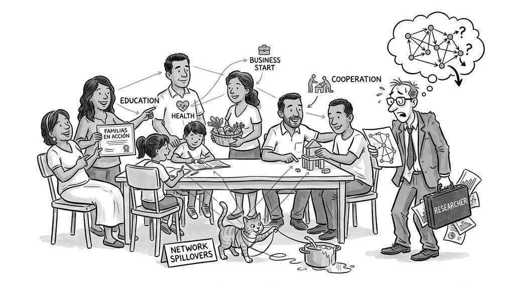
Researchers at the Inter-American Development Bank used heterogeneous treatment effect estimation combined with network spillover analysis to evaluate Colombia's conditional cash transfer program, Familias en Accion. By estimating CATEs across municipalities and mapping inter-municipality migration networks, the evaluation suggested that program effects on school enrollment were approximately 40% larger in municipalities with high network exposure to other treated municipalities, consistent with substantial spillover channels that a standard ATE analysis would have missed.
The Cobra Effect: When Policy Analyzers Would Have Helped
In colonial Delhi, the British government offered a bounty for dead cobras to reduce the snake population. Enterprising residents began breeding cobras for the reward. When officials discovered the scheme and scrapped the bounty, breeders released their now-worthless snakes, making the problem worse than before. This is a textbook case of missing the "who is harmed" analysis: a policy with a positive average effect (fewer wild cobras initially) concealed a subpopulation (breeders) whose behavioral response reversed the intended outcome. A heterogeneous treatment effect analysis with agent-based simulation could, in principle, have flagged the perverse incentive before deployment, provided the model included behavioral responses to the bounty structure.
Lab: Spillover Sensitivity Explorer
Goal: Empirically measure how the spillover coefficient changes the total policy effect and its distribution across network positions.
Tools needed: Python with numpy, pandas, networkx, econml, and matplotlib (approximately 20 minutes).
Procedure: Using the synthetic job training data from this section (or generating your own with 1,000 agents), run the PolicyImpactAnalyzer with five different spillover coefficients: 0.0, 0.1, 0.3, 0.5, and 0.8. For each run, record (a) the mean cumulative effect after 24 periods, (b) the Gini coefficient of outcomes, and (c) the mean outcome specifically for untreated agents.
What to vary: The spillover_coefficient parameter and, separately, the network topology (try Watts-Strogatz with rewiring probabilities 0.01, 0.1, and 0.5 to move from lattice-like to random-like graphs).
What to observe: Plot the mean untreated-agent outcome against spillover coefficient for each network type. You should typically observe that higher spillover amplifies the total effect but also tends to increase inequality (higher Gini), though the magnitude depends on the network's degree distribution. More random networks (higher rewiring) spread spillovers more evenly, reducing the Gini for the same spillover coefficient. Identify the combination of spillover and network structure where untreated agents benefit most relative to treated agents, as this reveals where indirect effects dominate direct ones.