"I simulated a universal basic income. The agents loved it. Then I gave them the ability to vote, and they abolished it to fund a space program. I had not programmed that."
A Mesa Model With Political Ambitions
Causal inference tells us what a policy did in the past. Policy simulation tells us what a policy would do in the future, under conditions that may differ from the historical setting. Agent-based models (ABMs) are uniquely suited to this task because they represent the heterogeneous, adaptive, interacting agents that make social systems hard to predict with aggregate equations. This section builds a complete agent-based economic simulation framework with Mesa, covering labor market dynamics, policy counterfactuals, calibration to empirical data, and the ethical constraints that govern experimentation on social systems.
1. From Equations to Agents
What. What happens to a city's labor market when the minimum wage doubles overnight? No government would run that experiment on real workers, but an agent-based economic model can: it represents the economy as a population of heterogeneous agents (workers, firms, consumers, regulators) that interact through markets, networks, and institutions. Each agent follows behavioral rules that may include optimization, heuristics, learning, and adaptation. Macro-level outcomes (unemployment rates, price distributions, inequality measures) emerge from micro-level interactions, letting analysts witness the consequences of untested policies before anyone's livelihood is at stake.
Why. Traditional economic models (Dynamic Stochastic General Equilibrium (DSGE), Computable General Equilibrium (CGE)) assume a "representative agent" that optimizes a well-defined objective function under rational expectations. This assumption makes the mathematics tractable but discards exactly the features that policy evaluation requires. It removes heterogeneity in how different groups respond to a policy and network effects that amplify or dampen shocks. It ignores adaptation that changes a policy's effectiveness over time and nonlinear dynamics that produce tipping points and regime shifts. ABMs sacrifice analytical tractability for representational fidelity.
How. We use Mesa, the Python agent-based modeling framework introduced in Section 43.1, extended with economic-specific components: labor markets, goods markets, monetary flows, and policy instruments. The counterfactual simulation pipeline (Figure 52.11) separates agent behavior (micro rules) from market mechanisms (matching and price formation) and policy instruments (taxes, transfers, regulations), allowing counterfactual analysis by swapping policy components while holding agent behavior fixed.
When. Use ABMs for policy simulation when (1) agent heterogeneity matters for the policy question, (2) network or spatial interactions mediate the policy effect, (3) agents adapt their behavior in response to the policy, or (4) you need to explore scenarios that have no historical precedent. For well-studied policies with established causal estimates, the empirical methods from Section 52.2 are often more credible; ABMs complement them by projecting effects into novel contexts. In short: run the same world twice, change one policy lever, and the difference between the two outcomes is your causal estimate.
The core value of an agent-based model for policy is not prediction but counterfactual comparison. You run the same model twice, once with the policy and once without, using the same random seed and initial conditions. The difference between the two runs isolates the causal effect of the policy within the model's logic. This is exactly the potential outcomes framework from Chapter 31, implemented computationally: the model generates both \(Y(0)\) and \(Y(1)\) for every agent, something that observational data can never provide. The credibility of the counterfactual depends entirely on the credibility of the model's behavioral rules.
Mental Model
Think of counterfactual policy analysis like a cooking experiment. You prepare two identical batches of bread dough from the same ingredients, weighed to the gram, at the same temperature. You bake one batch at 350 degrees and the other at 400 degrees. Because everything except the oven temperature is identical, any difference in the final loaves (crustiness, rise, moisture) must be caused by the temperature change alone. The shared random seed in an ABM serves the same role as the identical dough: it ensures that every agent makes the same sequence of "random" decisions in both runs, so the only source of divergence is the policy intervention you changed. Without the shared seed, you would be comparing bread made on different days with different flour, unable to tell whether the crust changed because of the temperature or because Tuesday's humidity was higher.
2. A Labor Market ABM with Mesa
The labor market simulation below models workers searching for jobs, firms posting vacancies, and a government implementing policy interventions. It serves as the simulation engine for the policy impact analyzer in Section 52.4.
import mesa
import numpy as np
from dataclasses import dataclass, field
from typing import Optional


@dataclass
class PolicyConfig:
    """Configuration for a policy intervention."""
    min_wage: float = 7.25
    training_subsidy: float = 0.0
    unemployment_benefit: float = 200.0
    hiring_tax_credit: float = 0.0
    training_duration: int = 4  # weeks


class Worker(mesa.Agent):
    """
    A worker agent who searches for jobs, accumulates skills,
    and responds to labor market policies.
    """

    def __init__(self, model, skill_level: float, sector: int):
        super().__init__(model)
        self.skill_level = skill_level
        self.sector = sector
        self.employed = False
        self.employer = None
        self.wage = 0.0
        self.savings = np.random.uniform(500, 5000)
        self.weeks_unemployed = 0
        self.in_training = False
        self.training_weeks_left = 0
        self.search_intensity = 1.0

    def step(self):
        if self.in_training:
            self._continue_training()
        elif self.employed:
            self._work()
        else:
            self._search_for_job()

    def _work(self):
        """Produce output, earn wage, update savings."""
        self.savings += self.wage
        self.weeks_unemployed = 0

        # Skill accumulation through learning-by-doing
        self.skill_level += 0.001 * self.model.random.random()

        # Exogenous separation risk
        if self.model.random.random() < 0.02:
            self.employer.remove_worker(self)
            self.employed = False
            self.employer = None
            self.wage = 0.0

    def _search_for_job(self):
        """Search for vacancies matching skills and sector."""
        self.weeks_unemployed += 1
        policy = self.model.policy

        # Collect unemployment benefit
        self.savings += policy.unemployment_benefit

        # Consider training if prolonged unemployment
        if (
            self.weeks_unemployed > 12
            and policy.training_subsidy > 0
            and not self.in_training
        ):
            if self.model.random.random() < 0.3:
                self.in_training = True
                self.training_weeks_left = policy.training_duration
                return

        # Search: sample vacancies, apply to best match
        vacancies = self.model.get_open_vacancies()
        if not vacancies:
            return

        n_applications = min(
            int(3 * self.search_intensity), len(vacancies)
        )
        sampled = self.model.random.sample(
            list(vacancies), n_applications
        )

        for firm in sampled:
            offered_wage = firm.offered_wage(self)
            if offered_wage >= max(
                policy.min_wage,
                policy.unemployment_benefit * 0.8
            ):
                # Accept the job
                firm.hire_worker(self, offered_wage)
                self.employed = True
                self.employer = firm
                self.wage = offered_wage
                break

        # Adjust search intensity based on duration
        self.search_intensity = max(
            0.5, 1.0 - 0.02 * self.weeks_unemployed
        )

    def _continue_training(self):
        """Participate in subsidized training program."""
        self.training_weeks_left -= 1
        self.savings += self.model.policy.training_subsidy

        if self.training_weeks_left <= 0:
            # Training complete: skill boost
            self.skill_level += 0.3 + 0.1 * self.model.random.random()
            self.in_training = False
            self.search_intensity = 1.0  # Renewed motivation


class Firm(mesa.Agent):
    """
    A firm agent that hires workers, produces output,
    and responds to labor market conditions.
    """

    def __init__(self, model, productivity: float, sector: int):
        super().__init__(model)
        self.productivity = productivity
        self.sector = sector
        self.workers: list = []
        self.revenue = 0.0
        self.vacancies = 0
        self.target_size = np.random.randint(3, 30)

    def step(self):
        self._produce()
        self._adjust_vacancies()

    def _produce(self):
        """Produce output based on workers' skills."""
        if not self.workers:
            self.revenue = 0.0
            return
        total_skill = sum(w.skill_level for w in self.workers)
        self.revenue = self.productivity * total_skill

    def _adjust_vacancies(self):
        """Post or withdraw vacancies based on profitability."""
        labor_cost = sum(w.wage for w in self.workers)
        profit = self.revenue - labor_cost

        if len(self.workers) < self.target_size and profit >= 0:
            self.vacancies = self.target_size - len(self.workers)
        else:
            self.vacancies = max(0, self.vacancies - 1)

    def offered_wage(self, worker: Worker) -> float:
        """
        Compute the wage offer for a candidate worker.
        Wage depends on worker skill, firm productivity,
        and the hiring tax credit.
        """
        base_wage = (
            self.productivity * worker.skill_level * 0.5
        )
        policy = self.model.policy
        # Tax credit lowers the firm's cost, enabling higher offers
        effective_wage = base_wage + policy.hiring_tax_credit
        return max(effective_wage, policy.min_wage)

    def hire_worker(self, worker: Worker, wage: float):
        self.workers.append(worker)
        self.vacancies = max(0, self.vacancies - 1)

    def remove_worker(self, worker: Worker):
        if worker in self.workers:
self.workers.remove(worker)class LaborMarketModel(mesa.Model):
"""
Agent-based labor market model for policy simulation.
Supports counterfactual analysis by running the same
initial conditions under different PolicyConfig settings.
"""
def __init__(
self,
n_workers: int = 1000,
n_firms: int = 100,
n_sectors: int = 4,
policy: PolicyConfig = None,
seed: int = 42,
):
super().__init__(seed=seed)
self.policy = policy or PolicyConfig()
self.n_sectors = n_sectors
# Create workers with heterogeneous skills
for _ in range(n_workers):
skill = max(0.1, np.random.lognormal(-0.5, 0.8))
sector = self.random.randrange(n_sectors)
Worker(self, skill_level=skill, sector=sector)
# Create firms with heterogeneous productivity
for _ in range(n_firms):
productivity = max(5.0, np.random.lognormal(2.5, 0.5))
sector = self.random.randrange(n_sectors)
Firm(self, productivity=productivity, sector=sector)
# Data collector for macro outcomes
self.datacollector = mesa.DataCollector(
model_reporters={
"unemployment_rate": self._unemployment_rate,
"mean_wage": self._mean_wage,
"wage_gini": self._wage_gini,
"mean_skill": self._mean_skill,
"total_output": self._total_output,
"training_enrollment": self._training_enrollment,
},
)
def step(self):
"""Advance the model by one time step (one week)."""
# Shuffle and step all agents
self.agents.shuffle_do("step")
self.datacollector.collect(self)
def get_open_vacancies(self) -> list:
"""Return firms with open vacancies."""
return [
a for a in self.agents_by_type[Firm]
if a.vacancies > 0
]
def _unemployment_rate(self) -> float:
workers = list(self.agents_by_type[Worker])
if not workers:
return 0.0
unemployed = sum(
1 for w in workers
if not w.employed and not w.in_training
)
return unemployed / len(workers)
def _mean_wage(self) -> float:
wages = [
w.wage for w in self.agents_by_type[Worker]
if w.employed
]
return np.mean(wages) if wages else 0.0
def _wage_gini(self) -> float:
wages = sorted([
w.wage for w in self.agents_by_type[Worker]
if w.employed and w.wage > 0
])
if len(wages) < 2:
return 0.0
n = len(wages)
cumulative = np.cumsum(wages)
return (
(2 * np.sum((np.arange(1, n + 1) * wages)))
/ (n * cumulative[-1])
- (n + 1) / n
)
def _mean_skill(self) -> float:
skills = [w.skill_level for w in self.agents_by_type[Worker]]
return np.mean(skills) if skills else 0.0
def _total_output(self) -> float:
return sum(f.revenue for f in self.agents_by_type[Firm])
def _training_enrollment(self) -> int:
return sum(
1 for w in self.agents_by_type[Worker] if w.in_training
)3. Counterfactual Policy Analysis
When Oregon expanded Medicaid by lottery in 2008, researchers gained a rare randomized policy experiment, but it took years and millions of dollars to measure the effects on a single state. Most proposed policies never get that luxury: no legislature will randomize a tax code change across cities just to generate clean data. Simulation-based counterfactuals fill that gap by letting analysts test policies that have no historical precedent and no ethical path to a real experiment.
The power of agent-based simulation lies in counterfactual comparison. As shown in Figure 52.11, we run the same model under two or more policy configurations, using identical random seeds and initial conditions, and attribute the difference in outcomes to the policy change. Figure 52.3.1 illustrates counterfactual policy simulation with paired random seeds.
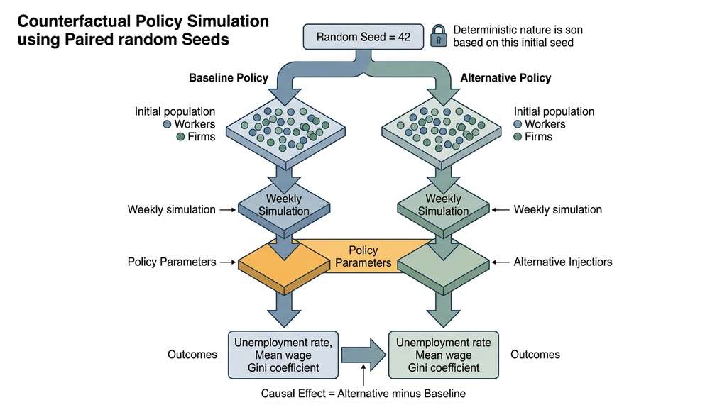
Counterfactual policy analysis estimates what would have happened under an alternative policy by comparing two simulation runs that differ only in the policy parameter of interest. Real-world policy experiments are expensive, slow, and often ethically impossible at scale, so simulation-based counterfactuals let analysts explore "what if" questions before committing public resources. Both runs share the same random seed, so every stochastic decision (which worker applies where, which firm experiences a demand shock) unfolds identically up to the point where the policy change forces a divergence. Any subsequent difference in macro outcomes traces back solely to that policy lever. Use counterfactual analysis over purely statistical approaches when you need to test policies with no historical precedent, examine interaction effects between multiple simultaneous changes, or trace the causal pathway from a policy lever to its aggregate effect at the agent level.
import pandas as pd


def run_counterfactual_analysis(
    baseline_policy: PolicyConfig,
    alternative_policy: PolicyConfig,
    n_steps: int = 52,
    n_replications: int = 10,
    n_workers: int = 1000,
    n_firms: int = 100,
) -> dict:
    """
    Run paired counterfactual simulations to estimate policy effects.

    Uses the same random seeds for baseline and alternative,
    ensuring that any difference in outcomes is attributable
    to the policy change alone.

    Parameters
    ----------
    baseline_policy : the status quo policy
    alternative_policy : the proposed policy change
    n_steps : simulation length (weeks)
    n_replications : number of independent runs for uncertainty

    Returns
    -------
    dict with per-step mean outcomes and confidence intervals
    """
    baseline_results = []
    alternative_results = []

    for rep in range(n_replications):
        seed = 1000 + rep  # Same seed for both runs

        # Baseline run
        model_b = LaborMarketModel(
            n_workers=n_workers, n_firms=n_firms,
            policy=baseline_policy, seed=seed,
        )
        for _ in range(n_steps):
            model_b.step()
        df_b = model_b.datacollector.get_model_dataframe()
        df_b["replication"] = rep
        df_b["policy"] = "baseline"
        baseline_results.append(df_b)

        # Alternative run (same seed, different policy)
        model_a = LaborMarketModel(
            n_workers=n_workers, n_firms=n_firms,
            policy=alternative_policy, seed=seed,
        )
        for _ in range(n_steps):
            model_a.step()
        df_a = model_a.datacollector.get_model_dataframe()
        df_a["replication"] = rep
        df_a["policy"] = "alternative"
        alternative_results.append(df_a)

    baseline_df = pd.concat(baseline_results)
    alternative_df = pd.concat(alternative_results)

    # Compute mean and CI for each metric at each step
    metrics = [
        "unemployment_rate", "mean_wage", "wage_gini",
        "mean_skill", "total_output",
    ]

    summary = {}
    for metric in metrics:
        b_mean = baseline_df.groupby(level=0)[metric].mean()
        a_mean = alternative_df.groupby(level=0)[metric].mean()
        b_std = baseline_df.groupby(level=0)[metric].std()
        a_std = alternative_df.groupby(level=0)[metric].std()

        effect = a_mean - b_mean
        effect_se = np.sqrt(
            (b_std ** 2 + a_std ** 2) / n_replications
        )

        summary[metric] = {
            "baseline_mean": b_mean.values,
            "alternative_mean": a_mean.values,
            "effect": effect.values,
            "effect_se": effect_se.values,
            "final_effect": effect.values[-1],
            "final_se": effect_se.values[-1],
        }

    return summary


# Compare: status quo vs. training subsidy program
baseline = PolicyConfig(
    min_wage=7.25, training_subsidy=0.0,
    unemployment_benefit=200.0, hiring_tax_credit=0.0,
)

training_program = PolicyConfig(
    min_wage=7.25, training_subsidy=150.0,
    unemployment_benefit=200.0, hiring_tax_credit=0.0,
    training_duration=8,
)

print("Running counterfactual analysis (10 replications)...")
effects = run_counterfactual_analysis(
    baseline, training_program,
    n_steps=52, n_replications=10,
    n_workers=500, n_firms=50,
)

for metric, data in effects.items():
    effect = data["final_effect"]
    se = data["final_se"]
    print(
        f"  {metric}: effect = {effect:+.4f} "
        f"(SE = {se:.4f})"
)Common Misconception
Readers often believe that a policy simulation's output is a forecast of what will happen in the real world. It is not. An ABM counterfactual tells you the causal effect of a policy within the model's own logic: if agents behave according to these rules and interact through these markets, then changing this policy lever produces that outcome difference. The result is only as credible as the behavioral rules and calibration. A model that omits informal labor markets, for example, will miss the channel through which many minimum wage effects actually operate. Treat simulation results as structured hypotheses to be tested against empirical evidence, never as direct predictions of real-world outcomes.
A state labor department uses the LaborMarketModel to evaluate a proposed minimum wage increase from \$7.25 to \$12.00. The simulation runs 20 replications of a 2-year horizon (104 weekly steps) with 5,000 workers and 500 firms calibrated to the state's industry mix. The counterfactual analysis reveals a nuanced effect: unemployment rises by 1.2 percentage points in the first quarter (firms slow hiring), then partially recovers as increased consumer spending raises demand. The Gini coefficient drops by 0.04, indicating reduced inequality. Workers in the bottom skill quintile experience 85% of the wage gains but also 60% of the job losses. The department uses these distributional breakdowns, not available from aggregate econometric models, to design a complementary retraining program targeted at the most vulnerable workers.
4. Calibration to Empirical Data
Counterfactual comparisons reveal detailed distributional effects, but their conclusions are only as trustworthy as the behavioral rules behind them. How do we ensure the model reflects the real economy?
An uncalibrated ABM is a thought experiment. A calibrated ABM is a testable hypothesis. Calibration adjusts model parameters so that simulated outcomes match observed empirical regularities, often called stylized facts (robust statistical patterns that hold across multiple datasets and time periods, such as a Beveridge curve relating vacancy rates to unemployment). Common targets include the unemployment rate, wage distribution shape, job duration distribution, and sectoral output shares.
from scipy.optimize import differential_evolution


def calibrate_model(
    empirical_targets: dict,
    n_steps: int = 52,
    n_replications: int = 5,
) -> dict:
    """
    Calibrate model parameters to match empirical targets
    using differential evolution (global optimization).

    Parameters
    ----------
    empirical_targets : dict mapping metric names to target values
        e.g., {"unemployment_rate": 0.05, "wage_gini": 0.35}

    Returns
    -------
    dict with calibrated parameters and fit quality
    """

    def objective(params):
        """
        Compute sum of squared relative errors between
        simulated and empirical targets.
        """
        n_workers_param = int(params[0])
        n_firms_param = int(params[1])
        min_wage = params[2]
        unemp_benefit = params[3]

        policy = PolicyConfig(
            min_wage=min_wage,
            unemployment_benefit=unemp_benefit,
        )

        total_error = 0.0
        for rep in range(n_replications):
            model = LaborMarketModel(
                n_workers=n_workers_param,
                n_firms=n_firms_param,
                policy=policy,
                seed=42 + rep,
            )
            for _ in range(n_steps):
                model.step()

            df = model.datacollector.get_model_dataframe()

            # Use the last 12 steps as steady-state
            steady_state = df.tail(12)

            for metric, target in empirical_targets.items():
                simulated = steady_state[metric].mean()
                if target != 0:
                    relative_error = (
                        (simulated - target) / target
                    ) ** 2
                else:
                    relative_error = simulated ** 2
                total_error += relative_error

        return total_error / n_replications

    # Parameter bounds
    bounds = [
        (200, 2000),    # n_workers
        (20, 200),      # n_firms
        (5.0, 15.0),    # min_wage
        (100.0, 500.0), # unemployment_benefit
    ]

    result = differential_evolution(
        objective, bounds, maxiter=50, seed=42,
        tol=1e-4, polish=True,
    )

    calibrated = {
        "n_workers": int(result.x[0]),
        "n_firms": int(result.x[1]),
        "min_wage": result.x[2],
        "unemployment_benefit": result.x[3],
        "fit_error": result.fun,
        "converged": result.success,
    }

    return calibrated


# Example calibration targets (US-like stylized facts)
targets = {
    "unemployment_rate": 0.05,
    "wage_gini": 0.35,
}

print("Calibrating model to empirical targets...")
print("(This may take several minutes for full optimization)")
# Uncomment to run: calibrated = calibrate_model(targets)Calibration ensures that your model reproduces the data you built it to match. Validation tests whether it reproduces data you did not build it to match. The strongest validation for a policy simulation model is to calibrate it on pre-policy data, then test whether it correctly predicts the outcomes of a policy change that has already been evaluated empirically (a "natural experiment"). If the model matches the known causal effect from a difference-in-differences or RD study (Section 52.2), it gains credibility for extrapolating to untested policy scenarios. This calibrate-then-validate cycle mirrors the train/test split in machine learning, applied to simulation models.
5. Ethical Constraints on Social Experimentation
Even a well-calibrated and validated model carries responsibilities beyond technical accuracy, because the systems it represents are composed of real people whose welfare is at stake.
Social and economic systems present ethical challenges that physical science simulations do not face. The agents in these systems are people. Experiments on them can cause real harm. Three principles constrain responsible policy simulation and experimentation.
Three Principles for Responsible Policy Simulation
Beneficence. Policy simulations should aim to improve outcomes for the affected population. A simulation that identifies a policy harming vulnerable subgroups has fulfilled its purpose by revealing the harm before implementation. The ethical obligation is to report distributional effects, not just average effects.
Non-maleficence. Even simulated policies can cause harm if they are implemented based on poorly validated models. The modeler bears responsibility for communicating uncertainty, disclosing model limitations, and distinguishing between robust findings (consistent across many calibrations) and fragile findings (sensitive to specific parameter choices).
Justice. Policy evaluations must examine heterogeneous effects across demographic groups, income levels, and geographic regions. A policy that improves the average while disproportionately burdening a minority group raises justice concerns that aggregate metrics conceal. The heterogeneous treatment effects from Section 52.2 and the agent-level distributional analysis in ABMs are essential tools for surfacing these concerns.
Checkpoint
So far: responsible policy simulation rests on three ethical principles: beneficence (aim to improve outcomes and report distributional effects), non-maleficence (communicate uncertainty and model limitations honestly), and justice (examine heterogeneous effects across demographic groups rather than relying on aggregate metrics alone).
Every modeling choice embeds a value judgment. Defining "unemployment" as a bad outcome assumes that all employment is good, regardless of quality. Choosing the Gini coefficient as the inequality measure weights transfers at different income levels differently than the Theil index (an entropy-based inequality measure that decomposes cleanly between and within subgroups) or the Palma ratio (the ratio of the richest 10% share of income to the poorest 40% share, emphasizing the tails of the distribution). Calibrating to GDP growth privileges aggregate output over distributional equity. The responsible modeler makes these choices explicit, tests sensitivity to alternative operationalizations, and presents results under multiple value frameworks rather than declaring a single "optimal" policy. This connects to the responsible AI discussion in Chapter 57.
def distributional_impact_analysis(
    model: LaborMarketModel,
    baseline_model: LaborMarketModel,
    skill_quantiles: int = 5,
) -> pd.DataFrame:
    """
    Analyze how a policy change affects different subgroups
    of the population, disaggregated by skill level.

    Parameters
    ----------
    model : the model run with the alternative policy
    baseline_model : the model run with baseline policy
    skill_quantiles : number of skill groups to analyze

    Returns
    -------
    DataFrame with per-group employment rate, mean wage,
    and mean savings changes
    """
    def extract_worker_data(m):
        return pd.DataFrame([
            {
                "skill": w.skill_level,
                "employed": w.employed,
                "wage": w.wage,
                "savings": w.savings,
                "weeks_unemployed": w.weeks_unemployed,
                "in_training": w.in_training,
            }
            for w in m.agents_by_type[Worker]
        ])

    alt_workers = extract_worker_data(model)
    base_workers = extract_worker_data(baseline_model)

    # Assign skill quantile groups
    skill_bins = pd.qcut(
        base_workers["skill"], skill_quantiles,
        labels=[f"Q{i+1}" for i in range(skill_quantiles)]
    )
    base_workers["skill_group"] = skill_bins
    alt_workers["skill_group"] = skill_bins

    # Compute group-level statistics
    groups = []
    for group in base_workers["skill_group"].unique():
        base_g = base_workers[base_workers["skill_group"] == group]
        alt_g = alt_workers[alt_workers["skill_group"] == group]

        groups.append({
            "skill_group": group,
            "n_workers": len(base_g),
            "baseline_employment": base_g["employed"].mean(),
            "alternative_employment": alt_g["employed"].mean(),
            "employment_change": (
                alt_g["employed"].mean() - base_g["employed"].mean()
            ),
            "baseline_mean_wage": base_g.loc[
                base_g["employed"], "wage"
            ].mean(),
            "alternative_mean_wage": alt_g.loc[
                alt_g["employed"], "wage"
            ].mean(),
            "wage_change": (
                alt_g.loc[alt_g["employed"], "wage"].mean()
                - base_g.loc[base_g["employed"], "wage"].mean()
            ),
            "savings_change": (
                alt_g["savings"].mean() - base_g["savings"].mean()
            ),
        })

    return pd.DataFrame(groups)


# Example distributional analysis
print("\nDistributional Impact by Skill Quintile:")
print("(Run after counterfactual simulation to see results)")
# dist = distributional_impact_analysis(model_alt, model_base)
# print(dist.to_string(index=False))The counterfactual analysis above required roughly 80 lines of custom orchestration code. Mesa's batch runner handles parameter sweeps, replications, and data collection in about 10 lines:
import mesa

# Define parameter space for policy experiments
params = {
    "n_workers": 500,
    "n_firms": 50,
    "policy": [
        PolicyConfig(min_wage=7.25),
        PolicyConfig(min_wage=10.00),
        PolicyConfig(min_wage=12.00),
        PolicyConfig(min_wage=15.00),
    ],
}

# Run batch experiment with 10 replications each
results = mesa.batch_run(
    LaborMarketModel, params,
    iterations=10, max_steps=52,
    data_collection_period=1,
)
results_df = pd.DataFrame(results)Mesa's batch_run handles seed management, parallel execution, and result aggregation internally, reducing the counterfactual analysis to a parameter specification problem. The 80 lines of custom code exist to show the paired-seed counterfactual logic that gives ABM experiments their causal interpretation.
6. Connecting Simulation to Causal Inference
The simulation framework in this section and the causal inference methods in Section 52.2 are complementary, not competing. Causal inference provides empirically grounded effect estimates that calibrate agent behavior. Simulation extends those estimates to novel contexts and untested policies. The policy impact analyzer in Section 52.4 combines both: it uses EconML's causal forest to estimate heterogeneous treatment effects from observational data, then embeds those effects as agent behavioral parameters in a Mesa simulation to project outcomes under counterfactual policy scenarios.
Research Frontier
Traditional ABM calibration requires hand-specifying agent behavioral rules, then tuning parameters to match aggregate data. A 2023 line of work on large language model (LLM) driven agents for economic simulation replaces hand-coded rules with LLM-generated behavior. Horton (2023), in "Large Language Models as Simulated Economic Agents," reported that GPT-4 agents reproducing classic behavioral economics experiments (ultimatum games, dictator games, labor supply decisions) approximately match human experimental results without task-specific calibration in the scenarios tested. The agents exhibit reference dependence, loss aversion, and status quo bias as emergent properties of language model reasoning rather than as programmed heuristics. More recently, the AgentTorch framework (Chopra et al., 2024) scales LLM-driven agents to populations of millions for pandemic and economic policy simulation, using a differentiable ABM architecture that back-propagates through both the simulation dynamics and a neural surrogate of agent behavior. These approaches do not eliminate the need for calibration and validation, but they shift the calibration target from dozens of behavioral parameters to the choice of prompt and model, raising new questions about what it means to "validate" agent behavior when the behavioral engine is a general-purpose language model.
Try It: Minimum Wage Dose-Response Curve
A dose-response curve (borrowed from pharmacology, where it maps drug dosage to biological effect) here maps the "dose" of a policy lever to the magnitude of an economic outcome, revealing diminishing returns and threshold effects.
Build a complete policy dose-response experiment that sweeps minimum wage levels and visualizes the tradeoff between employment and inequality. You need only Mesa, NumPy, pandas, and matplotlib.
Step 1. Copy the PolicyConfig, Worker, Firm, and LaborMarketModel classes from Figures 52.12 and 52.13 into a file called labor_abm.py.
Step 2. Write a sweep script that creates a list of seven PolicyConfig objects with minimum wages ranging from \$5.00 to \$20.00 in \$2.50 increments, holding all other parameters at their defaults.
Step 3. For each policy, run the model for 52 steps with 5 replications (seeds 100 through 104) and 500 workers / 50 firms. After each run, record the mean unemployment rate and mean Gini coefficient over the final 12 steps.
Step 4. Aggregate results across replications to compute the mean and standard deviation of both metrics at each wage level. Store these in a pandas DataFrame with columns: min_wage, unemp_mean, unemp_std, gini_mean, gini_std.
Step 5. Plot a dual-axis chart: unemployment rate (left y-axis) and Gini coefficient (right y-axis) as functions of the minimum wage (x-axis), with shaded error bands showing one standard deviation. Identify the "sweet spot" where the Gini drops substantially before unemployment rises sharply. This is the core tradeoff that policymakers navigate, and your chart makes it concrete.
Exercise 52.3.1
Suppose you run two counterfactual simulations of the LaborMarketModel: one with unemployment_benefit=200 and one with unemployment_benefit=400, both using seed 42 and 500 workers for 52 steps. In the high-benefit run, you observe that the unemployment rate rises by 2 percentage points but the wage_gini drops by 0.03. A colleague claims the higher benefit "caused unemployment." Identify at least two mechanisms in the model code (Figures 52.12 and 52.13) through which a higher unemployment benefit could raise the measured unemployment rate, and explain why one of those mechanisms might actually represent a positive outcome for workers despite increasing the headline number.
Hint
Look at the job acceptance condition in_search_for_job: workers reject offers below unemployment_benefit * 0.8. Also consider the training enrollment branch, which triggers after 12 weeks of unemployment. A higher benefit raises the reservation wage (the lowest wage a worker will accept, below which remaining unemployed yields higher utility), meaning fewer bad jobs are accepted. It also funds longer search or training spells, both of which increase measured unemployment but may improve match quality and long-run skill levels.Step-Through: Paired-Seed Counterfactual Logic
Trace through run_counterfactual_analysis for a single replication (rep=0) with 3 workers, 1 firm, and 4 steps to see why the shared seed matters.
Setup. Seed = 1000. Both baseline (min_wage=7.25) and alternative (min_wage=12.00) models are initialized with the same seed, so all three workers get identical skill draws: Worker A (skill 0.42), Worker B (skill 1.13), Worker C (skill 0.67). The single firm has productivity 14.2 and target_size 3.
Step 1. The random shuffle orders agents as [B, C, A, Firm]. In both runs, B searches first. The firm offers B a wage of 14.2 * 1.13 * 0.5 = 8.02. Baseline: 8.02 > 7.25, B accepts. Alternative: 8.02 < 12.00, B is rejected (offer below min_wage). First divergence.
Step 2. C searches. Firm offers 14.2 * 0.67 * 0.5 = 4.76. Baseline: 4.76 < 7.25, C rejects. Alternative: 4.76 < 12.00, C also rejects. Both runs agree: C stays unemployed.
Step 3. A searches. Firm offers 14.2 * 0.42 * 0.5 = 2.98. Both runs: 2.98 < min_wage, A rejects.
Step 4. Firm adjusts vacancies. Baseline: 1 worker hired, revenue = 14.2 * 1.13 = 16.05, vacancies remain 2. Alternative: 0 workers hired, revenue = 0, vacancies unchanged.
Result after 4 steps. Baseline unemployment = 2/3 = 66.7%. Alternative unemployment = 3/3 = 100%. The 33.3 pp difference is the estimated effect of raising the minimum wage to \$12.00 in this tiny economy. Because both runs used seed 1000, the same shuffle and the same skill draws occurred; the only source of divergence was the policy parameter.
Real-World Application: Bank of England CANVAS Model
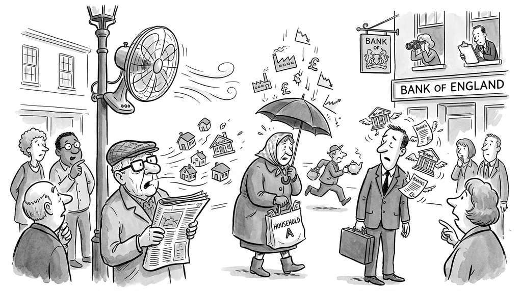
The Bank of England's CANVAS (Central Bank Agent-based Model for Vulnerabilities Assessment), as described in published Bank of England staff working papers, uses an agent-based simulation with heterogeneous households, firms, and banks to stress-test macroprudential policies before implementation. CANVAS reportedly calibrates agent behavioral rules to UK microdata (the Wealth and Assets Survey and Companies House filings), then runs paired counterfactuals to estimate how proposed loan-to-value caps or countercyclical capital buffers propagate through the credit network. The distributional breakdowns by income decile and region are intended to inform the Financial Policy Committee's decisions, illustrating how the Mesa-style counterfactual framework in this section can scale to national-level policy evaluation.
The Schelling Surprise That Launched a Field
Thomas Schelling's 1971 segregation model, one of the earliest agent-based social simulations, produced a result so counterintuitive that it changed how economists think about emergent phenomena. Schelling placed agents on a checkerboard and gave each a mild preference for having at least one-third of their neighbors be the same type. The result: near-complete segregation, far exceeding anything individual preferences would suggest. The lesson, that micro-level tolerance can produce macro-level intolerance, would have been difficult to derive from aggregate equations alone, because the emergent segregation pattern depends on spatial interactions that closed-form models typically abstract away. It was the simulation that made the invisible visible. Every modern policy ABM, including the labor market model in this section, inherits Schelling's core insight: aggregate outcomes are not simply scaled-up versions of individual behavior.
Lab: Policy Dose-Response Surface
Goal. Map the two-dimensional tradeoff surface between a minimum wage increase and a training subsidy, measuring unemployment and wage inequality as joint outcomes.
Tools. Python 3.10+, Mesa (pip install mesa), NumPy, pandas, matplotlib or seaborn.
Setup (5 min). Copy the PolicyConfig, Worker, Firm, and LaborMarketModel classes from Figures 52.12 and 52.13 into a single script. Create a grid of 5 minimum wage values (\$7.25, \$9, \$11, \$13, \$15) crossed with 4 training subsidy levels (\$0, \$75, \$150, \$225), giving 20 policy configurations.
Experiment (15 min). For each configuration, run 3 replications (seeds 0, 1, 2) with 300 workers, 30 firms, and 52 steps. Record the mean unemployment rate and Gini coefficient over the final 12 steps.
What to vary. The two policy levers (min_wage and training_subsidy). Hold worker count, firm count, simulation length, and all other PolicyConfig fields constant.
What to observe. Plot a heatmap (or contour plot) with minimum wage on the x-axis, training subsidy on the y-axis, and color representing (a) unemployment rate and (b) Gini coefficient. Look for a "valley" in the surface where unemployment stays low while inequality drops. Does the training subsidy shift the point at which minimum wage increases begin to destroy jobs? Compare the joint-policy optimum to the single-lever optima from the dose-response curve in the "Try It" exercise above.