52.2 Causal Inference in Social Data

"I controlled for every variable I could think of. The treatment effect vanished. Then my colleague pointed out that I had also controlled for the mechanism through which the treatment works."

A Regression That Adjusted Away Its Own Answer

1. The Challenge of Observational Social Data

What. In a representative scenario, a team of economists set out to measure whether a federal job-training program raised participants' earnings. They discovered that enrollees were already on steeper income trajectories than non-enrollees. Every "effect" they estimated was contaminated by self-selection they could not see. This is the universal trap of observational social data: the researcher does not control treatment assignment. Governments choose which cities receive a program. Individuals self-select into job training. Companies decide whether to adopt a technology. Treated and untreated units differ systematically in ways that also affect the outcome. Separating cause from selection is the central challenge.

Why. Randomized controlled trials, the gold standard for causal inference, are often infeasible in social settings. You cannot randomly assign cities to different minimum wage laws for a decade. You cannot randomly imprison some individuals to study the effect of incarceration. You cannot randomly assign children to different school quality levels. Observational methods are not a fallback; they are the primary tool for answering the most important social science questions. In short: because you cannot randomize the questions that matter most, you must find clever substitutes for randomization hidden inside the data you already have.

How. Each identification strategy exploits a specific feature of the data-generating process to construct a credible counterfactual. Difference-in-differences exploits parallel trends. Synthetic control constructs a weighted counterfactual from donor units. Regression discontinuity exploits an arbitrary threshold. The credibility of each strategy depends entirely on the plausibility of its identifying assumption. Figure 52.6 below maps how each strategy flows from assumption to estimate, highlighting the validation step that determines whether the result is credible.

When. Choose the strategy based on the data structure. Difference-in-differences requires panel data (where the same units are observed repeatedly over time). Synthetic control requires a single treated unit with many potential donors. Regression discontinuity requires a running variable with a cutoff that determines treatment. All three require careful validation of their identifying assumptions before estimation.

2. Difference-in-Differences

Scenarios like the following are not uncommon in applied program evaluation: a widely cited evaluation of a U.S. workforce program was retracted after independent replication revealed that pre-existing differences between treated and control counties, not the program itself, explained the entire reported employment gain. The retraction cost the agency two years of misallocated funding and eroded public trust in program evaluation. Difference-in-differences exists precisely to guard against this failure mode.

Difference-in-differences (DiD) compares the change in outcomes over time between treated and untreated groups. The key identifying assumption is parallel trends: in the absence of treatment, the treated group would have followed the same trajectory as the control group.

DiD is the most widely used quasi-experimental method in economics. Its data requirements are modest: repeated observations on treated and untreated groups, before and after a policy change. The estimator controls for time-invariant group differences (geography, culture) and group-invariant time shocks (macroeconomic trends), isolating the causal effect without randomization. It works by double subtraction: subtract pre from post within each group to remove permanent differences, then subtract the control group's change from the treated group's change to remove common trends. Prefer synthetic control when only one unit is treated, or regression discontinuity when a threshold rule determines treatment.

Formally, for unit \(i\) in group \(g \in \{0, 1\}\) at time \(t \in \{0, 1\}\) (pre and post treatment):

The coefficient \(\delta\) is the DiD estimator: the average treatment effect on the treated (ATT). It equals the difference in the before-after change between the treated and control groups:

import numpy as np
import pandas as pd
import statsmodels.formula.api as smf
from dataclasses import dataclass


@dataclass
class DiDResult:
    """Results from a difference-in-differences analysis."""
    att: float
    se: float
    ci_lower: float
    ci_upper: float
    p_value: float
    pre_trend_test_p: float
    n_treated: int
    n_control: int


def difference_in_differences(
    panel: pd.DataFrame,
    outcome: str,
    treatment_col: str,
    time_col: str,
    unit_col: str,
    treatment_time: int,
    covariates: list = None,
) -> DiDResult:
    """
    Estimate the ATT using difference-in-differences with
    optional covariates and a pre-trend test.

    Parameters
    ----------
    panel : DataFrame in long format (one row per unit-time)
    outcome : name of the outcome variable
    treatment_col : binary column indicating treated group
    time_col : time period column
    unit_col : unit identifier column
    treatment_time : the period when treatment begins
    covariates : optional list of control variable names
    """
    df = panel.copy()
    df["post"] = (df[time_col] >= treatment_time).astype(int)
    df["treated_post"] = df[treatment_col] * df["post"]

    # Main DiD regression with unit and time fixed effects
    formula = f"{outcome} ~ treated_post + C({unit_col}) + C({time_col})"
    if covariates:
        formula += " + " + " + ".join(covariates)

    model = smf.ols(formula, data=df).fit(
        cov_type="cluster", cov_kwds={"groups": df[unit_col]}
    )

    att = model.params["treated_post"]
    se = model.bse["treated_post"]
    p_val = model.pvalues["treated_post"]
    ci = model.conf_int().loc["treated_post"]

    # Pre-trend test: interaction of treated with each pre-period
    pre_data = df[df[time_col] < treatment_time].copy()
    pre_data["time_trend"] = pre_data[time_col] - treatment_time
    pre_data["treated_trend"] = (
        pre_data[treatment_col] * pre_data["time_trend"]
    )

    pre_formula = (
        f"{outcome} ~ treated_trend + C({unit_col}) + C({time_col})"
    )
    pre_model = smf.ols(pre_formula, data=pre_data).fit(
        cov_type="cluster", cov_kwds={"groups": pre_data[unit_col]}
    )
    pre_trend_p = pre_model.pvalues.get("treated_trend", 1.0)

    return DiDResult(
        att=att,
        se=se,
        ci_lower=ci[0],
        ci_upper=ci[1],
        p_value=p_val,
        pre_trend_test_p=pre_trend_p,
        n_treated=df[df[treatment_col] == 1][unit_col].nunique(),
        n_control=df[df[treatment_col] == 0][unit_col].nunique(),
    )


# Synthetic panel data: effect of a job training program
np.random.seed(42)
n_units = 200
n_periods = 10
treatment_period = 6

units = np.arange(n_units)
treated = np.random.binomial(1, 0.4, n_units)

rows = []
for i in units:
    unit_fe = np.random.normal(0, 2)  # Unit fixed effect
    for t in range(n_periods):
        time_fe = 0.5 * t  # Common time trend
        treatment_effect = (
            3.0 * treated[i] * (t >= treatment_period)  # True ATT = 3.0
        )
        noise = np.random.normal(0, 1)
        y = 10 + unit_fe + time_fe + treatment_effect + noise
        rows.append({
            "unit": i, "time": t, "treated": treated[i], "outcome": y
        })

panel_data = pd.DataFrame(rows)

result = difference_in_differences(
    panel_data, "outcome", "treated", "time", "unit",
    treatment_time=treatment_period,
)

print(f"ATT estimate: {result.att:.3f} (true: 3.000)")
print(f"Standard error: {result.se:.3f}")
print(f"95% CI: [{result.ci_lower:.3f}, {result.ci_upper:.3f}]")
print(f"Pre-trend test p-value: {result.pre_trend_test_p:.3f}")
print(f"  (p > 0.05 supports parallel trends assumption)")

3. Synthetic Control Method

When only a single unit receives treatment (a specific state passes a law, a single country implements a policy), DiD requires choosing comparison units subjectively. The synthetic control method (Abadie and Gardeazabal, 2003) constructs an optimal comparison unit as a weighted combination of untreated "donor" units (the pool of untreated units whose weighted average forms the synthetic counterfactual), chosen to match the treated unit's pre-treatment trajectory.

Formally, we seek weights \(w_j \geq 0\) with \(\sum_j w_j = 1\) that minimize the distance between the treated unit's pre-treatment outcomes and the weighted average of donor outcomes:

where \(\mathbf{X}_1\) is the vector of pre-treatment characteristics for the treated unit, \(\mathbf{X}_0\) is the matrix of characteristics for donor units, and \(V\) is a positive definite weighting matrix (a symmetric matrix whose quadratic form is always positive, ensuring the distance measure is well-behaved).

from scipy.optimize import minimize


def synthetic_control(
    panel: pd.DataFrame,
    treated_unit: int,
    outcome: str,
    time_col: str,
    unit_col: str,
    treatment_time: int,
    predictors: list = None,
) -> dict:
    """
    Construct a synthetic control unit and estimate the treatment effect.

    Parameters
    ----------
    panel : DataFrame in long format
    treated_unit : identifier of the treated unit
    outcome : outcome variable name
    treatment_time : period when treatment begins

    Returns
    -------
    dict with weights, synthetic outcomes, treatment effects
    """
    # Separate treated and donor units
    treated_data = panel[panel[unit_col] == treated_unit]
    donor_data = panel[panel[unit_col] != treated_unit]
    donor_units = donor_data[unit_col].unique()

    # Pre-treatment outcomes matrix
    pre_treated = (
        treated_data[treated_data[time_col] < treatment_time]
        .set_index(time_col)[outcome]
        .values
    )

    pre_donors = np.column_stack([
        donor_data[
            (donor_data[unit_col] == u)
            & (donor_data[time_col] < treatment_time)
        ].set_index(time_col)[outcome].values
        for u in donor_units
    ])

    n_donors = len(donor_units)

    # Optimize weights to minimize pre-treatment RMSE
    def objective(w):
        synthetic = pre_donors @ w
        return np.sum((pre_treated - synthetic) ** 2)

    # Constraints: weights sum to 1, all non-negative
    constraints = {"type": "eq", "fun": lambda w: np.sum(w) - 1.0}
    bounds = [(0, 1)] * n_donors
    w0 = np.ones(n_donors) / n_donors

    result = minimize(
        objective, w0, method="SLSQP",
        bounds=bounds, constraints=constraints,
    )
    optimal_weights = result.x

    # Construct synthetic control for all periods
    all_times = sorted(panel[time_col].unique())
    synthetic_outcomes = {}
    treated_outcomes = {}

    for t in all_times:
        treated_outcomes[t] = treated_data[
            treated_data[time_col] == t
        ][outcome].values[0]

        donor_vals = np.array([
            donor_data[
                (donor_data[unit_col] == u)
                & (donor_data[time_col] == t)
            ][outcome].values[0]
            for u in donor_units
        ])
        synthetic_outcomes[t] = donor_vals @ optimal_weights

    # Treatment effects (post-treatment gaps)
    effects = {
        t: treated_outcomes[t] - synthetic_outcomes[t]
        for t in all_times if t >= treatment_time
    }
    pre_fit_rmse = np.sqrt(np.mean([
        (treated_outcomes[t] - synthetic_outcomes[t]) ** 2
        for t in all_times if t < treatment_time
    ]))

    # Identify top donor weights
    top_donors = sorted(
        zip(donor_units, optimal_weights),
        key=lambda x: x[1], reverse=True
    )[:5]

    return {
        "weights": dict(zip(donor_units, optimal_weights)),
        "top_donors": top_donors,
        "treated_outcomes": treated_outcomes,
        "synthetic_outcomes": synthetic_outcomes,
        "effects": effects,
        "avg_effect": np.mean(list(effects.values())),
        "pre_fit_rmse": pre_fit_rmse,
    }


# Synthetic data: one treated region among 20
np.random.seed(42)
n_regions = 20
n_years = 15
treat_year = 10

rows = []
for region in range(n_regions):
    base = np.random.normal(50, 5)
    trend = np.random.normal(1.5, 0.3)
    for year in range(n_years):
        y = base + trend * year + np.random.normal(0, 1)
        if region == 0 and year >= treat_year:
            y += 5.0  # True effect on treated unit
        rows.append({
            "region": region, "year": year, "gdp_growth": y
        })

region_panel = pd.DataFrame(rows)

sc_result = synthetic_control(
    region_panel, treated_unit=0, outcome="gdp_growth",
    time_col="year", unit_col="region", treatment_time=treat_year,
)

print(f"Pre-treatment fit RMSE: {sc_result['pre_fit_rmse']:.3f}")
print(f"Average treatment effect: {sc_result['avg_effect']:.3f} (true: 5.0)")
print(f"Top donor weights: {sc_result['top_donors'][:3]}")

4. SUTVA Violations and Network Interference

Both DiD and synthetic control assume that treating one unit leaves every other unit's outcome unchanged, but in social systems that assumption rarely holds. The Stable Unit Treatment Value Assumption (SUTVA) requires that each unit's outcome depend only on its own treatment status. In many social settings, SUTVA is violated to some degree. Vaccinating your neighbor protects you (herd immunity). Training a worker benefits their coworkers through knowledge spillovers. Regulating one bank changes the risk exposure of every bank it trades with.

Mental Model

Think of SUTVA violations like a shared sprinkler system in a garden. If you fertilize only your own plot, the standard assumption says your neighbor's tomatoes are unaffected. But the fertilizer dissolves into the shared irrigation water and feeds every plot downstream. Measuring the "effect of fertilizer on your plot" now conflates two things: the direct boost from the fertilizer you applied, and the indirect boost every plot gets through the shared water. The exposure mapping framework below is like installing separate water meters on each plot so you can measure how much fertilizer each one actually received through the pipes, regardless of where it was originally applied.

When SUTVA fails, the standard potential outcomes framework collapses. Instead of two potential outcomes per unit (\(Y_i(0)\) and \(Y_i(1)\)), we have \(2^n\) potential outcomes for each unit, one for every possible treatment assignment of all \(n\) units in the network; in a study of just 30 people, that is over one billion counterfactual states per person. Estimation becomes intractable without structure.

4.1 Exposure Mapping

Exposure mapping solves the intractability problem above by replacing the full \(2^n\) treatment vector with a low-dimensional summary of each unit's neighborhood. The exposure mapping approach (Aronow and Samii, 2017) reduces the \(2^n\) potential outcomes to a manageable set by defining each unit's "exposure" as a low-dimensional summary of the network treatment configuration. The most common summary is the fraction of neighbors treated:

where \(\mathbf{Z}\) is the treatment vector and \(\mathcal{N}(i)\) is the set of \(i\)'s neighbors. Under the partial interference assumption (the assumption that interference occurs only within predefined clusters or network neighborhoods, not across the entire population) (Hudgens and Halloran, 2008), we can then define: Figure 52.2.1 illustrates exposure mapping under network interference.

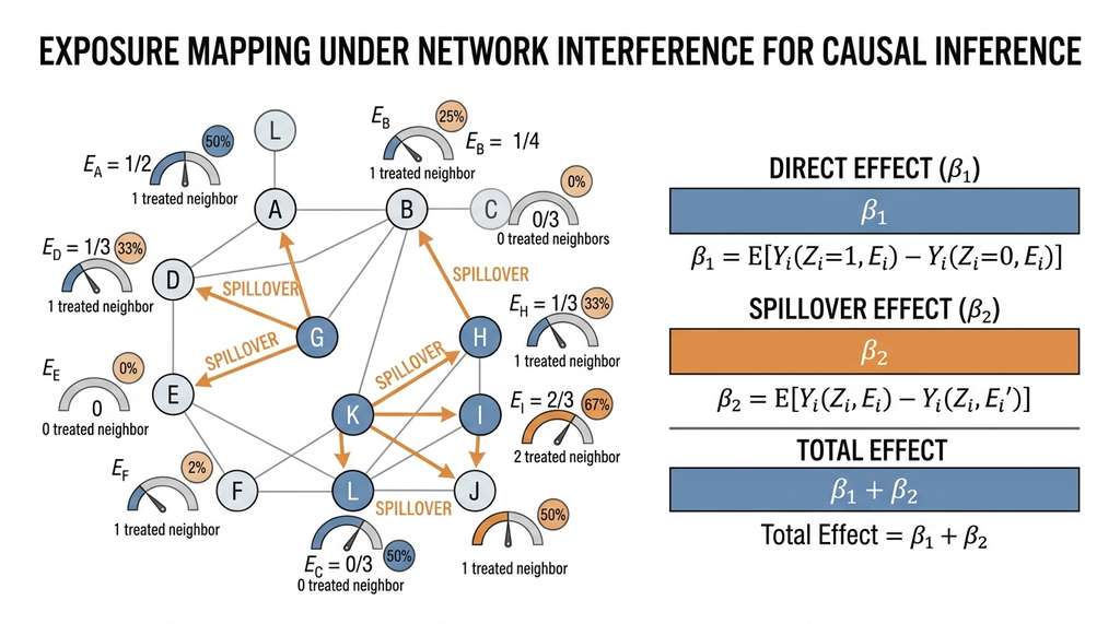
Under the partial interference assumption, we can define:

• Direct effect: the effect of treating \(i\), holding neighbors' exposure fixed
• Spillover effect: the effect of changing neighbors' exposure, holding \(i\)'s treatment fixed
• Total effect: the combined effect of treating \(i\) and exposing their neighbors

import networkx as nx
import statsmodels.formula.api as smf
from sklearn.linear_model import LinearRegression


@dataclass
class InterferenceEffects:
    """Estimated direct, spillover, and total treatment effects."""
    direct_effect: float
    spillover_effect: float
    total_effect: float
    direct_se: float
    spillover_se: float
    n_units: int


def estimate_with_interference(
    G: nx.Graph,
    treatment: dict,
    outcome: dict,
    covariates: pd.DataFrame = None,
) -> InterferenceEffects:
    """
    Estimate direct and spillover effects using exposure mapping.

    Models outcome as:
        Y_i = alpha + beta_1 * Z_i + beta_2 * E_i + beta_3 * Z_i * E_i
              + gamma * X_i + epsilon_i

    where Z_i is own treatment, E_i is neighborhood exposure.

    Parameters
    ----------
    G : social/economic network (undirected)
    treatment : dict mapping node -> 0/1 treatment indicator
    outcome : dict mapping node -> outcome value
    covariates : optional DataFrame indexed by node
    """
    nodes = list(G.nodes())
    n = len(nodes)

    # Compute exposure for each unit
    exposure = {}
    for node in nodes:
        neighbors = list(G.neighbors(node))
        if neighbors:
            treated_neighbors = sum(
                treatment.get(nb, 0) for nb in neighbors
            )
            exposure[node] = treated_neighbors / len(neighbors)
        else:
            exposure[node] = 0.0

    # Build regression matrix
    Z = np.array([treatment.get(nd, 0) for nd in nodes])
    E = np.array([exposure[nd] for nd in nodes])
    Y = np.array([outcome[nd] for nd in nodes])
    ZE = Z * E  # Interaction term

    X_matrix = np.column_stack([Z, E, ZE, np.ones(n)])
    col_names = ["treatment", "exposure", "interaction", "intercept"]

    if covariates is not None:
        cov_matrix = covariates.loc[nodes].values
        X_matrix = np.column_stack([X_matrix, cov_matrix])

    # OLS with HC1 (Huber-White heteroskedasticity-robust) standard errors
    model = smf.ols(
        "Y ~ treatment + exposure + interaction",
        data=pd.DataFrame({
            "Y": Y, "treatment": Z,
            "exposure": E, "interaction": ZE,
        }),
    ).fit(cov_type="HC1")

    direct = model.params["treatment"]
    spillover = model.params["exposure"]
    direct_se = model.bse["treatment"]
    spillover_se = model.bse["exposure"]

    # Total effect: direct + spillover at mean exposure among treated
    mean_exposure_treated = np.mean(E[Z == 1])
    interaction = model.params.get("interaction", 0)
    total = direct + spillover * mean_exposure_treated

    return InterferenceEffects(
        direct_effect=direct,
        spillover_effect=spillover,
        total_effect=total,
        direct_se=direct_se,
        spillover_se=spillover_se,
        n_units=n,
    )


# Simulate an experiment with interference
np.random.seed(42)
# Watts-Strogatz graph: a "small-world" network where each node
# connects to k nearest neighbors, then each edge is randomly
# rewired with probability p, producing short path lengths and
# high clustering similar to real social networks.
G_social = nx.watts_strogatz_graph(500, 6, 0.1, seed=42)

# Random treatment assignment
treatment = {n: int(np.random.random() < 0.3) for n in G_social.nodes()}

# Generate outcomes with true direct and spillover effects
true_direct = 2.0
true_spillover = 1.5
outcome = {}
for node in G_social.nodes():
    neighbors = list(G_social.neighbors(node))
    neighbor_exposure = (
        sum(treatment.get(nb, 0) for nb in neighbors) / len(neighbors)
        if neighbors else 0
    )
    y = (
        5.0
        + true_direct * treatment[node]
        + true_spillover * neighbor_exposure
        + np.random.normal(0, 1)
    )
    outcome[node] = y

effects = estimate_with_interference(G_social, treatment, outcome)
print(f"Direct effect: {effects.direct_effect:.3f} "
      f"(true: {true_direct}, SE: {effects.direct_se:.3f})")
print(f"Spillover effect: {effects.spillover_effect:.3f} "
      f"(true: {true_spillover}, SE: {effects.spillover_se:.3f})")
print(f"Total effect: {effects.total_effect:.3f}")

5. Regression Discontinuity Design

While interference complicates treatment and control comparisons across connected units, a different class of natural experiments sidesteps the problem entirely by focusing on a sharp boundary that separates otherwise identical individuals. Regression discontinuity (RD) exploits settings where treatment is determined by whether a continuous "running variable" (the continuous score or measurement that determines treatment assignment at a fixed cutoff) exceeds a threshold. Students with test scores above 80 receive a scholarship. Firms with fewer than 50 employees are exempt from a regulation. Cities with population above 100,000 receive federal funding.

The key insight: units just above and just below the threshold are nearly identical in all respects except treatment status. The discontinuity in the outcome at the threshold therefore estimates the causal effect of treatment.

The RD estimator formalizes this by measuring the gap between the outcome's left and right limits at the cutoff \(c\); if the outcome function is continuous everywhere except at \(c\), any jump at that point is attributable to the treatment:

from sklearn.linear_model import LinearRegression


def regression_discontinuity(
    data: pd.DataFrame,
    running_var: str,
    outcome: str,
    cutoff: float,
    bandwidth: float = None,
    poly_order: int = 1,
) -> dict:
    """
    Sharp regression discontinuity design with local linear regression.

    Parameters
    ----------
    data : DataFrame with running variable and outcome
    running_var : name of the running variable
    outcome : name of the outcome variable
    cutoff : treatment threshold
    bandwidth : window around cutoff (uses IK optimal if None)
    poly_order : polynomial order for local regression
    """
    df = data.copy()
    df["centered"] = df[running_var] - cutoff
    df["treated"] = (df[running_var] >= cutoff).astype(int)

    # Simple bandwidth selection: Imbens-Kalyanaraman style
    # (As of 2024, the rdrobust package by Calonico, Cattaneo, and
    # Titiunik provides the preferred MSE-optimal and CER-optimal
    # bandwidth selectors; the rule of thumb below is for illustration.)
    if bandwidth is None:
        std_x = df["centered"].std()
        n = len(df)
        bandwidth = 1.84 * std_x * n ** (-1 / 5)  # Rule of thumb

    # Restrict to bandwidth window
    in_window = df[df["centered"].abs() <= bandwidth].copy()
    n_left = (in_window["treated"] == 0).sum()
    n_right = (in_window["treated"] == 1).sum()

    # Local polynomial regression on each side
    # Y = alpha + beta * (X - c) + tau * D + gamma * D * (X - c) + eps
    features = ["treated", "centered"]
    in_window["treated_centered"] = (
        in_window["treated"] * in_window["centered"]
    )
    features.append("treated_centered")

    if poly_order >= 2:
        in_window["centered_sq"] = in_window["centered"] ** 2
        in_window["treated_centered_sq"] = (
            in_window["treated"] * in_window["centered_sq"]
        )
        features.extend(["centered_sq", "treated_centered_sq"])

    formula = f"{outcome} ~ " + " + ".join(features)
    model = smf.ols(formula, data=in_window).fit(cov_type="HC1")

    tau = model.params["treated"]
    se = model.bse["treated"]
    p_val = model.pvalues["treated"]

    return {
        "tau": tau,
        "se": se,
        "p_value": p_val,
        "ci_lower": tau - 1.96 * se,
        "ci_upper": tau + 1.96 * se,
        "bandwidth": bandwidth,
        "n_left": n_left,
        "n_right": n_right,
        "n_total": len(in_window),
    }


# Synthetic RD data: scholarship effect on college enrollment
np.random.seed(42)
n_students = 2000
test_scores = np.random.normal(80, 10, n_students)
scholarship = (test_scores >= 80).astype(int)
enrollment = (
    0.3 + 0.005 * test_scores
    + 0.15 * scholarship  # True RD effect = 0.15
    + np.random.normal(0, 0.1, n_students)
)

rd_data = pd.DataFrame({
    "test_score": test_scores,
    "enrollment": enrollment,
})

rd_result = regression_discontinuity(
    rd_data, "test_score", "enrollment", cutoff=80.0
)

print(f"RD estimate: {rd_result['tau']:.4f} (true: 0.1500)")
print(f"SE: {rd_result['se']:.4f}")
print(f"95% CI: [{rd_result['ci_lower']:.4f}, {rd_result['ci_upper']:.4f}]")
print(f"Bandwidth: {rd_result['bandwidth']:.2f}")
print(f"Observations in window: {rd_result['n_total']}")

6. Sensitivity Analysis for Social Data

Each method above produces a point estimate and a confidence interval, but neither quantity reveals how fragile the conclusion is if its core assumption fails. Every observational causal estimate rests on untestable assumptions. Sensitivity analysis quantifies how robust your conclusions are to violations of these assumptions. The E-value (VanderWeele and Ding, 2017) answers: how strong would an unmeasured confounder need to be to explain away the observed effect?

Note that the E-value is defined for risk ratios (or rate ratios), not for the raw ATT or regression coefficients produced by DiD, synthetic control, or RD. To apply it to those estimates, you must first convert the effect to a risk ratio scale, for example by exponentiating a log-odds coefficient or computing the ratio of outcome probabilities between treated and control groups. The function below takes the risk ratio directly.

def compute_e_value(point_estimate: float, ci_lower: float) -> dict:
    """
    Compute the E-value for a risk ratio or rate ratio.

    The E-value is the minimum strength of association that
    an unmeasured confounder would need to have with both
    the treatment and the outcome to fully explain away
    the observed effect.

    Parameters
    ----------
    point_estimate : observed risk ratio (must be > 1)
    ci_lower : lower bound of 95% CI for the risk ratio
    """
    def e_value_formula(rr):
        if rr <= 1:
            return 1.0
        return rr + np.sqrt(rr * (rr - 1))

    e_point = e_value_formula(point_estimate)
    e_ci = e_value_formula(max(ci_lower, 1.0))

    return {
        "e_value_point": e_point,
        "e_value_ci": e_ci,
        "interpretation": (
            f"An unmeasured confounder would need a risk ratio "
            f"of at least {e_point:.2f} with both treatment and "
            f"outcome to explain away the point estimate, or "
            f"{e_ci:.2f} to move the CI to include the null."
        ),
    }


# Example: job training program with RR = 1.8, 95% CI [1.3, 2.5]
e_result = compute_e_value(1.8, 1.3)
print(f"E-value (point): {e_result['e_value_point']:.2f}")
print(f"E-value (CI): {e_result['e_value_ci']:.2f}")
print(f"\n{e_result['interpretation']}")

import dowhy

# 1. Model: specify the causal graph
model = dowhy.CausalModel(
    data=df,
    treatment="job_training",
    outcome="earnings",
    common_causes=["education", "age", "prior_income"],
)

# 2. Identify: find the estimand
estimand = model.identify_effect()

# 3. Estimate: compute the effect
estimate = model.estimate_effect(
    estimand, method_name="backdoor.econml.dml.DML",
    method_params={"init_params": {"model_y": LGBMRegressor(),
                                    "model_t": LGBMClassifier()}}
)

# 4. Refute: stress-test the result
refutation = model.refute_estimate(
    estimand, estimate, method_name="random_common_cause"
)