"I mapped every handshake at the conference. By lunch, I could predict who would co-author a paper, who would co-found a startup, and who would never speak again."
A Social Network That Knew Too Much
When Lehman Brothers filed for bankruptcy in September 2008, the initial loss was \$639 billion, but the damage that followed was \$10 trillion: the shock raced through a web of lending relationships that nobody had fully mapped, toppling institutions three and four links away from the original failure. The structure of that network, not the attributes of any single bank, determined who survived and who collapsed. This section builds the network analysis toolkit for social and economic discovery: constructing graphs from relational data, measuring the structural importance of actors, detecting community structure for market segmentation, and modeling influence diffusion to understand adoption and contagion. Figure 52.7 illustrates the full pipeline from raw relational data to discovery insights.
1. Social and Economic Networks as Graphs
What. A social or economic network is a graph \(G = (V, E)\) where vertices \(V\) represent actors (people, firms, countries, products) and edges \(E\) represent relationships (trade, communication, citation, influence). Edges may be directed (A cites B), weighted (trade volume between countries), signed (trust or distrust), or temporal (the relationship exists during a specific period).
Why. Network structure shapes outcomes in ways that actor-level attributes alone cannot explain. A firm's position in a supply chain determines its vulnerability to disruption. A person's location in a social network determines how quickly they receive information. A bank's connections determine whether its failure triggers a systemic cascade. Ignoring network structure means ignoring the mechanism through which many social and economic phenomena operate.
How. We represent networks as graph objects using NetworkX (a Python library for creating, manipulating, and analyzing graphs), attaching node and edge attributes that encode economic and social variables. The graph then serves as the substrate for centrality analysis, community detection, and diffusion simulation.
When. Use network analysis whenever the relationships between actors matter as much as the attributes of the actors themselves. This includes supply chain analysis, financial contagion modeling, technology adoption studies, labor market analysis, and any setting where "who knows whom" or "who trades with whom" determines outcomes.
1.1 Building Economic Networks with NetworkX
The following code constructs a realistic inter-firm trade network from transaction data. Each firm is a node; each directed edge represents a buyer-seller relationship weighted by trade volume. In short: the graph is not a visualization convenience; it is the causal plumbing through which economic shocks, innovations, and information actually travel.
import networkx as nx
import numpy as np
import pandas as pd


def build_trade_network(transactions: pd.DataFrame) -> nx.DiGraph:
    """
    Build a directed trade network from transaction records.

    Parameters
    ----------
    transactions : DataFrame with columns
        'buyer_id', 'seller_id', 'amount', 'sector', 'date'

    Returns
    -------
    nx.DiGraph with node attributes (sector, total_volume)
        and edge attributes (weight, transaction_count)
    """
    G = nx.DiGraph()

    # Aggregate transactions by buyer-seller pair
    edge_data = (
        transactions.groupby(["buyer_id", "seller_id"])
        .agg(
            weight=("amount", "sum"),
            transaction_count=("amount", "count"),
            first_trade=("date", "min"),
            last_trade=("date", "max"),
        )
        .reset_index()
    )

    # Add edges with attributes
    for _, row in edge_data.iterrows():
        G.add_edge(
            row["buyer_id"],
            row["seller_id"],
            weight=row["weight"],
            transaction_count=row["transaction_count"],
            first_trade=row["first_trade"],
            last_trade=row["last_trade"],
        )

    # Add node attributes from firm metadata
    firm_sectors = transactions.drop_duplicates("buyer_id")[
        ["buyer_id", "sector"]
    ]
    for _, row in firm_sectors.iterrows():
        if row["buyer_id"] in G:
            G.nodes[row["buyer_id"]]["sector"] = row["sector"]

    # Compute total trade volume per node
    for node in G.nodes():
        in_volume = sum(
            d["weight"] for _, _, d in G.in_edges(node, data=True)
        )
        out_volume = sum(
            d["weight"] for _, _, d in G.out_edges(node, data=True)
        )
        G.nodes[node]["total_volume"] = in_volume + out_volume

    return G


# Example: synthetic trade data for demonstration
np.random.seed(42)
n_firms = 200
n_transactions = 2000

synthetic_transactions = pd.DataFrame({
    "buyer_id": np.random.randint(0, n_firms, n_transactions),
    "seller_id": np.random.randint(0, n_firms, n_transactions),
    "amount": np.random.lognormal(10, 2, n_transactions),
    "sector": np.random.choice(
        ["tech", "finance", "manufacturing", "retail"],
        n_transactions
    ),
    "date": pd.date_range("2023-01-01", periods=n_transactions, freq="h"),
})

# Remove self-loops
synthetic_transactions = synthetic_transactions[
    synthetic_transactions["buyer_id"] != synthetic_transactions["seller_id"]
]

trade_network = build_trade_network(synthetic_transactions)
print(f"Nodes: {trade_network.number_of_nodes()}")
print(f"Edges: {trade_network.number_of_edges()}")
print(f"Density: {nx.density(trade_network):.4f}")The network representation is not merely a convenient data structure. It encodes the mechanism through which economic effects propagate. When we later estimate causal effects in Section 52.2, the network determines which units interfere with each other. When we simulate policy in Section 52.3, the network determines which agents interact. The graph is the theory of how the system works, connecting back to the "executable theory" perspective from Section 43.1.
2. Centrality Measures for Market Structure
In 2011, flooding in Thailand knocked out a single hard-drive component supplier that few outside the industry had heard of. Because that firm sat on the only short path between two major manufacturing clusters, global hard-drive prices reportedly doubled within weeks and took over a year to fully recover. A five-minute centrality calculation on the supply network would have flagged the vulnerability before the waters rose.
Centrality measures quantify the structural importance of nodes in a network. In economic networks, centrality identifies systemically important firms, key intermediaries in supply chains, and influential actors in markets. Different centrality measures capture different notions of importance.
A centrality measure assigns a single numerical score to each node in a graph. It ranks nodes by structural importance according to a specific criterion. A node's score often predicts real outcomes: how fast it receives information, how resilient it is to removal, and how strongly it can influence others. Each centrality measure formalizes a different intuition about importance (number of connections, control over shortest paths, recursive prestige from neighbors). The right choice depends on the question you are asking. Use degree centrality when raw connectivity is the quantity of interest, betweenness when you care about brokerage and gatekeeping, and eigenvector or PageRank when influence flows recursively through the network.
Degree centrality counts connections: \(C_D(v) = \frac{\deg(v)}{n - 1}\). In a trade network, high in-degree means many suppliers (diversified sourcing); high out-degree means many customers (broad market reach).
Betweenness centrality measures brokerage: \(C_B(v) = \sum_{s \neq v \neq t} \frac{\sigma_{st}(v)}{\sigma_{st}}\), where \(\sigma_{st}\) is the number of shortest paths from \(s\) to \(t\) and \(\sigma_{st}(v)\) is the number passing through \(v\). High betweenness identifies firms that bridge otherwise disconnected market segments. In empirical trade networks, the rank correlation between degree and betweenness centrality is typically below 0.4, meaning the most connected firms and the most critical brokers tend to be largely different sets of actors.
Checkpoint
So far: a network is a graph of actors and relationships; degree centrality counts raw connections, while betweenness centrality identifies brokers who control shortest paths between other actors.
Recursive and Global Measures
Eigenvector centrality measures influence: a node is important if it is connected to other important nodes. The centrality vector \(\mathbf{x}\) satisfies \(A\mathbf{x} = \lambda \mathbf{x}\) where \(A\) is the adjacency matrix and \(\lambda\) is the leading eigenvalue. Google's PageRank is a damped variant designed for directed graphs.
Katz centrality accounts for all walks, not just shortest paths: \(C_K(v) = \sum_{k=1}^{\infty} \sum_{j=1}^{n} \alpha^k (A^k)_{jv}\), where \(\lambda_1\) is the largest eigenvalue of \(A\) and \(\alpha < 1/\lambda_1\) ensures convergence. This captures indirect influence that flows through long chains of intermediaries.
Mental Model
Think of centrality measures as different ways to rank airports. Degree centrality counts direct flights: O'Hare has many. Betweenness centrality identifies transfer hubs: if most passengers must connect through Dallas to get from the Southeast to the West Coast, Dallas has high betweenness even if it has fewer total flights than O'Hare. Eigenvector centrality rewards being connected to other well-connected airports: a regional airport with a single flight to Heathrow scores higher than one with five flights to small cities. Just as no single airport ranking captures "most important" without context, no single centrality measure captures structural importance universally. The choice depends on whether you care about connectivity, brokerage, or recursive prestige.
def analyze_market_structure(G: nx.DiGraph) -> pd.DataFrame:
    """
    Compute multiple centrality measures to identify
    structurally important actors in an economic network.
    """
    # Compute centralities
    degree_cent = nx.degree_centrality(G)
    in_degree_cent = nx.in_degree_centrality(G)
    out_degree_cent = nx.out_degree_centrality(G)
    betweenness_cent = nx.betweenness_centrality(G, weight="weight")
    pagerank = nx.pagerank(G, weight="weight", alpha=0.85)

    # For eigenvector centrality on directed graphs, use left eigenvector
    try:
        eigenvector_cent = nx.eigenvector_centrality_numpy(G, weight="weight")
    except nx.NetworkXException:
        eigenvector_cent = {n: 0.0 for n in G.nodes()}

    # Assemble results
    results = pd.DataFrame({
        "degree": degree_cent,
        "in_degree": in_degree_cent,
        "out_degree": out_degree_cent,
        "betweenness": betweenness_cent,
        "pagerank": pagerank,
        "eigenvector": eigenvector_cent,
    })

    # Rank correlation between measures reveals structural properties
    rank_corr = results.rank().corr(method="spearman")

    return results, rank_corr


centrality_df, rank_correlations = analyze_market_structure(trade_network)

# Identify systemically important firms (top 5% by PageRank)
threshold = centrality_df["pagerank"].quantile(0.95)
systemic_firms = centrality_df[
    centrality_df["pagerank"] >= threshold
].sort_values("pagerank", ascending=False)

print(f"Systemically important firms: {len(systemic_firms)}")
print(f"\nCentrality rank correlations:\n{rank_correlations.round(3)}")A logistics company analyzes its supplier network with 15,000 firms and 45,000 trade relationships. Betweenness centrality reveals that three small component manufacturers, individually accounting for less than 0.1% of total trade volume, serve as the sole bridge between two major manufacturing clusters. PageRank, which emphasizes volume, misses these firms entirely. The company identifies these "thin bridges" as single points of failure and negotiates backup supplier agreements, preventing a disruption that would have halted production across both clusters when one bridge firm later goes bankrupt.
3. Community Detection for Market Segmentation
Centrality measures rank individual actors by structural importance, but markets are not shaped by isolated players alone; they are organized into clusters of tightly interacting firms whose collective behavior defines market segments.
Community detection partitions a network into groups of densely connected nodes, revealing the natural segments of a market. In trade networks, communities often correspond to industry clusters, geographic regions, or supply chain tiers. The modular structure tells us where market boundaries lie and which firms bridge separate market segments.
The standard objective is modularity maximization. Modularity \(Q\) measures whether a partition has more intra-community edges than expected under a random null model:
$$Q = \frac{1}{2m} \sum_{ij} \left[ A_{ij} - \frac{k_i k_j}{2m} \right] \delta(c_i, c_j)$$where \(m\) is the total number of edges, \(k_i\) is the degree of node \(i\), \(c_i\) is the community assignment of node \(i\), and \(\delta\) is the Kronecker delta (a function that equals 1 when its two arguments are equal and 0 otherwise, so only pairs of nodes in the same community contribute to the sum).
Common Misconception
A frequent mistake is assuming that high modularity means the detected communities are "real" groups with meaningful economic identity. Modularity optimization can produce high scores on completely random networks, and many distinct partitions of the same network may yield nearly identical modularity values (the so-called "degeneracy" problem). Communities are statistical patterns of dense connectivity relative to a null model, not necessarily meaningful market segments. Always validate detected communities against external evidence (sector labels, geographic data, known industry groupings) before treating them as ground-truth market boundaries.
import networkx.algorithms.community as nx_comm


def detect_market_segments(G: nx.DiGraph, resolution: float = 1.0):
    """
    Detect market segments using the Louvain algorithm
    on the undirected projection of the trade network.

    Parameters
    ----------
    G : directed trade network
    resolution : higher values produce more, smaller communities

    Returns
    -------
    dict mapping node -> community_id, modularity score
    """
    # Convert to undirected for community detection
    G_undirected = G.to_undirected()

    # Louvain community detection (greedy modularity optimization)
    communities = nx_comm.louvain_communities(
        G_undirected, weight="weight", resolution=resolution, seed=42
    )

    # Build node -> community mapping
    node_to_community = {}
    for idx, community in enumerate(communities):
        for node in community:
            node_to_community[node] = idx

    # Compute modularity
    modularity = nx_comm.modularity(
        G_undirected, communities, weight="weight"
    )

    # Characterize each community
    community_stats = []
    for idx, community in enumerate(communities):
        subgraph = G.subgraph(community)
        internal_volume = sum(
            d["weight"] for _, _, d in subgraph.edges(data=True)
        )
        community_stats.append({
            "community_id": idx,
            "size": len(community),
            "internal_edges": subgraph.number_of_edges(),
            "internal_volume": internal_volume,
            "density": nx.density(subgraph),
        })

    return node_to_community, modularity, pd.DataFrame(community_stats)


communities, Q, community_stats = detect_market_segments(trade_network)
print(f"Communities found: {len(community_stats)}")
print(f"Modularity: {Q:.4f}")
print(f"\nCommunity statistics:\n{community_stats.head(10)}")Modularity optimization has a well-known resolution limit (Fortunato and Barthelemy, 2007): communities smaller than \(\sqrt{2m}\) edges may be merged into larger groups even when they are clearly distinct. For large economic networks, this means fine-grained market niches may be invisible to modularity-based methods. Use the resolution parameter to explore multiple scales, or consider hierarchical methods like the Leiden algorithm (an improved variant of Louvain that guarantees well-connected communities and avoids poorly connected intermediate partitions) that provide multi-resolution community structure. (As of 2024, NetworkX includes leiden_communities directly, making the Leiden algorithm a drop-in replacement for Louvain without requiring a separate library such as leidenalg.)
4. Influence Diffusion and Adoption Models
Centrality and community structure describe the static architecture of a network, but markets are dynamic: shocks propagate, innovations spread, and behaviors cascade from node to node along the very edges we have been measuring.
How does a new technology, a financial shock, or a policy change spread through a social or economic network? Diffusion models formalize this process. Two canonical models from Kempe, Kleinberg, and Tardos (2003) provide the foundation.
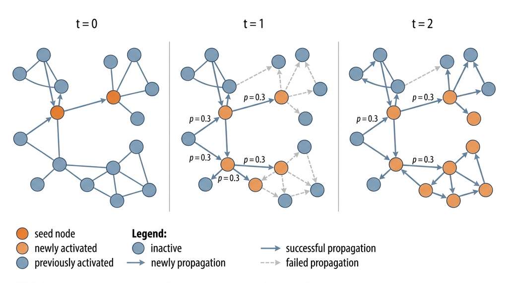
Independent Cascade (IC). Each newly activated node \(v\) gets one chance to activate each inactive neighbor \(w\) with probability \(p_{vw}\). The process runs until no new activations occur. This models information spread, viral adoption, and financial contagion where each exposure is an independent "trial." Figure 52.1.1 illustrates Independent Cascade influence diffusion on a network.
Linear Threshold (LT). Each node \(v\) has a threshold \(\theta_v\) drawn uniformly from \([0, 1]\). Node \(v\) activates when the total weight of its active neighbors exceeds \(\theta_v\): \(\sum_{w \in \text{active neighbors}} b_{wv} \geq \theta_v\), where \(b_{wv}\) is the influence weight of neighbor \(w\) on node \(v\) (typically derived from the edge weight normalized by \(v\)'s total incoming weight). This models adoption decisions where cumulative social pressure matters.
def independent_cascade(
    G: nx.DiGraph,
    seed_nodes: set,
    propagation_prob: float = 0.1,
    max_steps: int = 100,
    rng: np.random.Generator = None,
) -> dict:
    """
    Simulate the Independent Cascade diffusion model.

    Returns
    -------
    dict with 'activated' (set of all activated nodes),
    'timeline' (list of sets, newly activated at each step),
    'total_reached' (int)
    """
    if rng is None:
        rng = np.random.default_rng(42)

    activated = set(seed_nodes)
    timeline = [set(seed_nodes)]
    newly_activated = set(seed_nodes)

    for step in range(max_steps):
        next_activated = set()
        for node in newly_activated:
            for neighbor in G.successors(node):
                if neighbor not in activated:
                    # Edge-specific probability from weight if available
                    edge_data = G[node][neighbor]
                    prob = edge_data.get("influence_prob", propagation_prob)
                    if rng.random() < prob:
                        next_activated.add(neighbor)

        if not next_activated:
            break

        activated.update(next_activated)
        newly_activated = next_activated
        timeline.append(next_activated)

    return {
        "activated": activated,
        "timeline": timeline,
        "total_reached": len(activated),
        "steps": len(timeline),
    }


def influence_maximization_greedy(
    G: nx.DiGraph,
    k: int,
    propagation_prob: float = 0.1,
    n_simulations: int = 100,
) -> list:
    """
    Greedy algorithm for influence maximization.
    Select k seed nodes that maximize expected spread
    under the Independent Cascade model.

    The greedy algorithm achieves a (1 - 1/e) approximation
    ratio due to submodularity of the influence function.
    """
    rng = np.random.default_rng(42)
    selected_seeds = []

    for i in range(k):
        best_node = None
        best_marginal = -1

        candidates = set(G.nodes()) - set(selected_seeds)
        for candidate in candidates:
            trial_seeds = set(selected_seeds) | {candidate}

            # Monte Carlo estimate of expected spread
            spreads = []
            for sim in range(n_simulations):
                result = independent_cascade(
                    G, trial_seeds, propagation_prob,
                    rng=np.random.default_rng(sim)
                )
                spreads.append(result["total_reached"])

            expected_spread = np.mean(spreads)
            if expected_spread > best_marginal:
                best_marginal = expected_spread
                best_node = candidate

        selected_seeds.append(best_node)
        print(
            f"  Seed {i+1}: node {best_node}, "
            f"expected spread: {best_marginal:.1f}"
        )

    return selected_seeds


# Run influence maximization on a smaller subgraph for speed
top_nodes = centrality_df.nlargest(50, "pagerank").index.tolist()
sub_network = trade_network.subgraph(top_nodes).copy()

print("Greedy influence maximization (k=3):")
seeds = influence_maximization_greedy(sub_network, k=3, n_simulations=50)The influence function \(\sigma(S)\) (expected number of activated nodes given seed set \(S\)) is submodular: adding a seed to a small set produces larger marginal gain than adding it to a large set. A function \(f\) is submodular when \(f(A \cup \{x\}) - f(A) \geq f(B \cup \{x\}) - f(B)\) for all \(A \subseteq B\); intuitively, each additional element contributes less as the set grows. This mathematical property guarantees that the greedy algorithm, which adds one seed at a time choosing the maximum marginal gain, achieves at least 63% of the optimal spread. No polynomial-time algorithm can do better unless P = NP. This is the same submodularity that appears in Chapter 46's treatment of experimental design, where submodular set functions guide the selection of informative experiments.
5. Spatial Economic Analysis with PySAL
The diffusion models above treat network topology as abstract connectivity, but in many economic settings the edges themselves are grounded in physical geography: trade decays with distance, property values cluster by neighborhood, and regional unemployment follows spatial contours.
PySAL (Python Spatial Analysis Library) addresses this spatial dependence with tools for autocorrelation testing, spatial regression, and geographic clustering. The spatial track in Figure 52.7 shows where this analysis fits within the broader pipeline.
import libpysal
from esda.moran import Moran
from spreg import OLS, ML_Lag


def spatial_market_analysis(
    locations: pd.DataFrame,
    outcome_col: str = "price",
    feature_cols: list = None,
    k_neighbors: int = 8,
):
    """
    Analyze spatial dependence in economic outcomes.

    Parameters
    ----------
    locations : DataFrame with columns 'x', 'y', outcome_col,
        and feature columns
    outcome_col : the economic outcome to analyze
    feature_cols : covariates for spatial regression
    k_neighbors : number of neighbors for spatial weights

    Returns
    -------
    dict with Moran's I statistic, spatial lag regression results
    """
    # Construct spatial weights (k-nearest neighbors)
    points = list(zip(locations["x"], locations["y"]))
    w = libpysal.weights.KNN.from_array(
        np.array(points), k=k_neighbors
    )
    w.transform = "r"  # Row-standardize: each row sums to 1, so neighbors contribute equally

    # Global spatial autocorrelation: Moran's I
    y = locations[outcome_col].values
    moran = Moran(y, w)

    results = {
        "morans_I": moran.I,
        "morans_p": moran.p_sim,
        "morans_z": moran.z_sim,
        "interpretation": (
            "Significant positive spatial autocorrelation"
            if moran.p_sim < 0.05 and moran.I > 0
            else "No significant spatial autocorrelation"
        ),
    }

    # Spatial lag model: y = rho * W * y + X * beta + epsilon
    if feature_cols:
        X = locations[feature_cols].values
        y_col = locations[[outcome_col]].values

        # OLS for comparison (ignores spatial dependence)
        ols_model = OLS(y_col, X, name_y=outcome_col, name_x=feature_cols)

        # Maximum likelihood spatial lag model
        lag_model = ML_Lag(
            y_col, X, w,
            name_y=outcome_col, name_x=feature_cols
        )

        results["ols_r2"] = ols_model.r2
        results["spatial_lag_r2"] = lag_model.pr2
        results["rho"] = lag_model.rho  # Spatial autoregressive parameter
        results["rho_p"] = lag_model.z_stat[-1][1]

    return results


# Synthetic spatial economic data
np.random.seed(42)
n_locations = 500
spatial_data = pd.DataFrame({
    "x": np.random.uniform(0, 100, n_locations),
    "y": np.random.uniform(0, 100, n_locations),
    "income": np.random.lognormal(10, 0.5, n_locations),
    "population": np.random.lognormal(8, 1, n_locations),
})

# Generate spatially correlated prices (nearby locations have similar prices)
from scipy.spatial.distance import cdist
coords = spatial_data[["x", "y"]].values
dist_matrix = cdist(coords, coords)
spatial_corr = np.exp(-dist_matrix / 20)  # Exponential decay
spatial_noise = spatial_corr @ np.random.randn(n_locations)
spatial_data["price"] = (
    50000 + 2.0 * spatial_data["income"]
    + 0.5 * spatial_data["population"]
    + 5000 * spatial_noise
)

results = spatial_market_analysis(
    spatial_data, "price", ["income", "population"]
)
print(f"Moran's I: {results['morans_I']:.4f} (p={results['morans_p']:.4f})")
print(f"OLS R-squared: {results['ols_r2']:.4f}")
print(f"Spatial Lag R-squared: {results['spatial_lag_r2']:.4f}")
print(f"Spatial autoregressive rho: {results['rho']:.4f}")The full pipeline above (network construction, centrality, community detection, spatial analysis) spans roughly 200 lines of custom code. With NetworkX and PySAL's high-level APIs, the core analysis collapses to about 10 lines:
import networkx as nx
from networkx.algorithms.community import louvain_communities
from esda.moran import Moran
import libpysal

# Network: build, compute centrality, detect communities
G = nx.from_pandas_edgelist(df, "buyer", "seller", ["amount"], nx.DiGraph)
pr = nx.pagerank(G, weight="amount")
comms = louvain_communities(G.to_undirected(), weight="amount", seed=42)

# Spatial: test autocorrelation
w = libpysal.weights.KNN.from_dataframe(gdf, k=8)
moran = Moran(gdf["price"], w)
print(f"Moran's I={moran.I:.3f}, p={moran.p_sim:.3f}")NetworkX handles graph construction, 15+ centrality algorithms, and community detection internally. PySAL handles spatial weights construction, autocorrelation testing, and spatial regression. The 200 lines above exist to show what these libraries compute and why each step matters for market discovery.
A financial regulator constructs a transaction network from blockchain data: 50,000 wallet addresses, 2.3 million transactions. PageRank identifies 12 wallets that collectively process 40% of all transaction volume. Community detection reveals five tightly connected clusters, each centered on a major exchange. Influence diffusion simulation shows that a liquidity shock at any one of the top-3 wallets propagates to 60% of the network within 4 hops. The regulator uses this analysis to design circuit breakers: if transaction velocity from a systemically important wallet exceeds 3 standard deviations from its 30-day mean, automatic monitoring triggers alert human reviewers.
6. Network Discovery for the Discovery Workbench
Together, centrality analysis, community detection, and influence diffusion transform raw relational data into actionable market discovery: identifying which actors hold structural power, where natural market boundaries lie, and how shocks or innovations will propagate. The network analysis tools in this section feed directly into the Discovery Workbench pipeline. The graph structure becomes an input to the causal inference methods of Section 52.2, where network position determines exposure to treatment spillovers. The community structure informs the agent-based simulations of Section 52.3, where agents within the same community interact more frequently. The centrality measures serve as features when Section 52.4 estimates heterogeneous treatment effects, letting the policy impact analyzer discover whether effects vary by structural position.
class NetworkDiscoveryModule:
    """
    Discovery Workbench component for network analysis.
    Produces a standardized network summary for downstream
    causal inference and simulation modules.
    """

    def __init__(self, graph: nx.DiGraph):
        self.graph = graph
        self._centralities = None
        self._communities = None

    def analyze(self) -> dict:
        """Run full network discovery pipeline."""
        # Centrality analysis
        self._centralities = {
            "pagerank": nx.pagerank(self.graph, weight="weight"),
            "betweenness": nx.betweenness_centrality(
                self.graph, weight="weight"
            ),
            "in_degree": nx.in_degree_centrality(self.graph),
        }

        # Community detection
        undirected = self.graph.to_undirected()
        communities = louvain_communities(
            undirected, weight="weight", seed=42
        )
        self._communities = {}
        for idx, comm in enumerate(communities):
            for node in comm:
                self._communities[node] = idx

        # Network-level summary statistics
        summary = {
            "n_nodes": self.graph.number_of_nodes(),
            "n_edges": self.graph.number_of_edges(),
            "density": nx.density(self.graph),
            "n_communities": len(communities),
            "avg_clustering": nx.average_clustering(undirected),
            "centralities": self._centralities,
            "community_assignments": self._communities,
        }

        return summary

    def get_exposure_features(self, treatment_assignment: dict) -> dict:
        """
        Compute network exposure features for causal inference.
        Used by Section 52.2's interference-aware estimators.
        """
        exposure = {}
        for node in self.graph.nodes():
            neighbors = list(self.graph.predecessors(node))
            if neighbors:
                treated_neighbors = sum(
                    1 for n in neighbors
                    if treatment_assignment.get(n, 0) == 1
                )
                exposure[node] = treated_neighbors / len(neighbors)
            else:
                exposure[node] = 0.0
return exposureResearch Frontier
Graph foundation models now extend the reach of network analysis beyond hand-crafted features. Mao et al. (2024), "Graph Foundation Models" (ICML 2024), demonstrate that a single graph transformer pretrained on diverse graph datasets (social, biological, molecular) can be fine-tuned for node classification, link prediction, and community detection on economic networks with as few as 50 labeled examples. This "pretrain once, fine-tune everywhere" paradigm replaces the need to select and compute centrality features manually, instead learning task-relevant structural representations directly from adjacency data. For market discovery, such models can identify latent structural roles (broker, hub, peripheral) that no single classical centrality measure captures, and they generalize across network domains without re-engineering the feature pipeline. For practitioners working at scale, PyTorch Geometric (PyG) and the Deep Graph Library (DGL) now provide production-grade graph neural network pipelines that handle networks with millions of nodes, complementing NetworkX's strengths on smaller, analysis-focused graphs.
Try It: Map Your Own Collaboration Network
Build and analyze a real collaboration network using publicly available data, requiring only Python, NetworkX, and matplotlib. (1) Install dependencies: pip install networkx matplotlib pandas. (2) Choose a data source: download a small edge list from the Stanford Network Analysis Project (SNAP) repository (snap.stanford.edu/data), such as the email-Eu-core dataset (~1,000 nodes, ~25,000 edges), and load it with G = nx.read_edgelist("email-Eu-core.txt"). (3) Compute three centrality measures (degree, betweenness, PageRank) and store them in a DataFrame; identify the top 10 nodes by each measure and note which nodes appear in multiple top-10 lists. (4) Run Louvain community detection with two different resolution values (0.5 and 2.0) and compare the number of communities found at each scale. (5) Visualize the network with nx.draw_spring(G, node_size=[v*3000 for v in pagerank.values()], node_color=list(community_map.values()), cmap=plt.cm.tab10), sizing nodes by PageRank and coloring by community. Compare your visualization to the centrality rankings: do the visually prominent nodes match the numerically top-ranked ones?
Exercise 52.1.1
Consider a directed trade network with five firms: A sells to B and C; B sells to C and D; C sells to D and E; D sells to E; E sells to A. All edge weights are equal. Without running code, determine which firm has the highest betweenness centrality and explain why. Then verify your answer by constructing the graph in NetworkX and calling nx.betweenness_centrality(G).
Hint
Betweenness centrality counts how many shortest paths pass through a node. Draw out all 20 directed shortest paths (one for each ordered pair of distinct nodes) and tally which intermediate nodes appear on each path. The node that sits on the most shortest paths wins. Pay attention to nodes that serve as the only bridge between otherwise distant pairs.Step-Through: Greedy Influence Maximization
Trace through the greedy algorithm on a tiny 5-node directed graph with edges A→B (p=0.5), A→C (p=0.3), B→D (p=0.4), C→D (p=0.6), D→E (p=0.8). We want k=2 seed nodes. Suppose each "expected spread" is estimated from 3 Monte Carlo runs.
Round 1: Evaluate each candidate as a lone seed. Seed={A}: cascade can reach B (p=0.5), C (p=0.3), then D, then E. Across 3 runs the expected spread averages 3.0. Seed={B}: can only reach D (p=0.4), then E (p=0.8). Average spread: 2.0. Seed={C}: reaches D (p=0.6), then E (p=0.8). Average spread: 2.3. Seed={D}: reaches only E (p=0.8). Average spread: 1.7. Seed={E}: no outgoing edges. Average spread: 1.0. Best marginal gain: A with 3.0. Select A.
Round 2: Seeds so far = {A}. Evaluate each remaining candidate added to {A}. Seed={A,C}: A already tends to reach B and sometimes C; adding C guarantees C is active, boosting the path C→D→E. Average spread: 4.0. Seed={A,B}: adding B guarantees B, boosting B→D→E. Average spread: 3.7. Seed={A,D}: average 3.3. Seed={A,E}: average 3.1. Best marginal gain: C with 4.0 − 3.0 = 1.0. Select C. Final seed set: {A, C}.
Real-World Application: JPMorgan's Network-Based Fraud Detection
JPMorgan Chase has reported using graph analytics on transaction networks to detect fraud rings that evade traditional rule-based systems. By constructing a directed graph of money flows between accounts and running community detection, the system identifies tightly connected clusters of accounts that exhibit coordinated behavior (rapid circular transfers, shared counterparties, synchronized timing). Accounts with anomalously high betweenness centrality between legitimate and suspicious clusters are flagged as potential money mule intermediaries, catching patterns that per-account monitoring misses entirely.
The Friendship Paradox: Your Friends Are More Popular Than You
In 1991, sociologist Scott Feld proved a startling mathematical fact: on average, your friends have more friends than you do. This is not a psychological illusion; it follows directly from network structure. High-degree nodes appear in many people's friend lists, biasing the sample upward. The result has practical consequences: during the 2009 H1N1 flu outbreak, researchers at Harvard exploited the friendship paradox to build an early warning system. Instead of monitoring random people, they asked random people to name a friend, then monitored those friends. Because the named friends were statistically more central in the social network, they caught the flu 2 weeks earlier than the random sample, providing a 14-day advance warning signal with no knowledge of the network's actual structure.
Lab: Influence Maximization Showdown
Goal: Compare greedy influence maximization against simple heuristics (highest degree, highest PageRank, random selection) on a real social network and measure which seed selection strategy achieves the greatest cascade spread.
Tools needed: Python, NetworkX, matplotlib. Download the "ego-Facebook" dataset from SNAP (snap.stanford.edu/data/ego-Facebook.html), which contains ~4,000 nodes and ~88,000 edges.
Procedure (25 minutes): (1) Load the graph and convert to directed by replacing each undirected edge with two directed edges. (2) Implement the Independent Cascade model with propagation probability p=0.02. (3) For k=5 seed nodes, select seeds using four strategies: top-5 by degree, top-5 by PageRank, 5 random nodes, and the greedy algorithm (use 20 Monte Carlo simulations per candidate for speed). (4) For each strategy, run 100 IC simulations and record the mean and standard deviation of cascade size.
What to vary: Try propagation probabilities p in {0.01, 0.02, 0.05, 0.1}. At which threshold does seed selection strategy stop mattering (because the cascade saturates the network regardless)?
What to observe: How close does the degree heuristic come to greedy? At low p values, does PageRank outperform degree? Plot cascade size distributions as box plots for each strategy and propagation probability.