46.2 Sequential Experimental Design

The sequential design loop, illustrated in Figure 46.3 below, repeats four stages: update the surrogate model (a statistical proxy for the expensive real experiment; defined fully below) with new observations, score every candidate experiment using an acquisition function, run the top-scoring experiment, and feed the result back into the model. Each pass through the loop tightens the posterior and steers the next experiment toward the region of the design space where information gain is greatest.

1. Information-Theoretic Acquisition Functions

In drug discovery, each cell viability assay costs hundreds of dollars; in materials science, fabricating a single alloy sample can take days. Choose the wrong experiment and you burn budget on a measurement that tells you nothing new. Choose well, and a dozen targeted experiments can outperform a hundred random ones. The difference comes down to a formal criterion for ranking candidates before any tube is filled or any furnace is lit.

You have budget for one more experiment, and a thousand candidates are waiting: which single measurement, out of all of them, would teach you the most about the system you are studying? To answer it, you need a scoring rule that ranks every candidate by the expected information it would deliver. That rule traces back to a single quantity: the mutual information between the experiment's outcome and the unknown variable you care about. Here \(\omega\) might be the model parameters \(\theta\), the optimal input \(x^*\), or the true function \(f\) itself. We formalize "uncertainty" as the entropy (a non-negative quantity that measures how spread out a probability distribution is; higher entropy means greater uncertainty) of the posterior distribution \(p(\omega \mid \mathcal{D})\) given data \(\mathcal{D}\).

An acquisition function assigns a numerical score to each candidate experiment, ranking candidates by expected usefulness. The system then picks the highest-scoring candidate as the next experiment to run. Acquisition functions matter because real experiments (synthesizing a molecule, running a clinical assay, fabricating a device) are expensive, and choosing poorly wastes budget on uninformative measurements. For every candidate experiment \(x\), the acquisition function simulates the posterior under each possible outcome \(y\), then averages the resulting improvement (in entropy, utility, or regret) over the predictive distribution of \(y\). Use an information-theoretic acquisition function when the goal is to learn a model or map a function globally. Switch to a bandit or Bayesian optimization acquisition function when the goal is to find the best input rather than to understand the full landscape. In short: the acquisition function is the compass of sequential design; it converts what you do not know into a single number that tells you what to measure next.

Entropy reduction. If we run experiment \(x\) and observe outcome \(y\), the posterior entropy changes from \(H[\omega \mid \mathcal{D}]\) to \(H[\omega \mid \mathcal{D} \cup \{(x, y)\}]\). Since we do not know \(y\) in advance, we take the expectation:

This quantity is precisely the mutual information between the outcome \(y\) and the quantity of interest \(\omega\), conditioned on the data and the experiment:

Mutual information is always non-negative (observing data never increases expected uncertainty) and is zero only when \(y\) and \(\omega\) are conditionally independent given \(\mathcal{D}\) (the experiment provides no information about \(\omega\)). Selecting \(x^* = \arg\max_x I(\omega; y \mid x, \mathcal{D})\) is the information-theoretically optimal design criterion.

2. BALD: Bayesian Active Learning by Disagreement

BALD (Houlsby et al., 2011) instantiates the mutual information criterion with \(\omega = \theta\) (the model parameters). For a Bayesian model with parameter posterior \(p(\theta \mid \mathcal{D})\), the BALD acquisition function is:

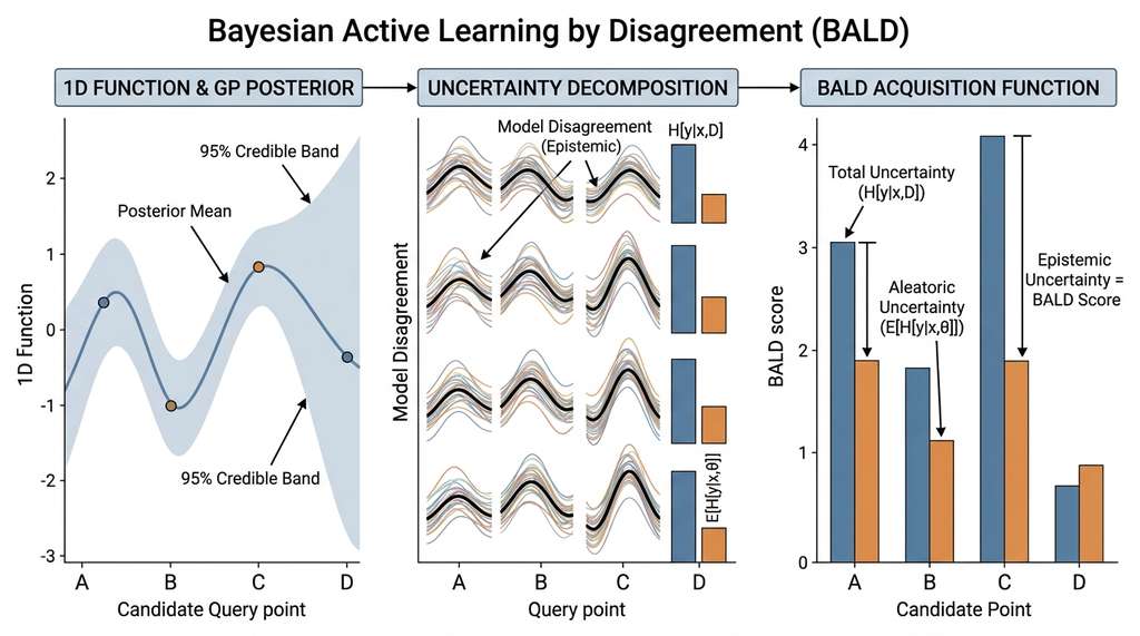
The first term, \(H[y \mid x, \mathcal{D}]\), is the entropy of the predictive distribution (the committee's average prediction, integrating over parameter uncertainty). The second term, \(\mathbb{E}_\theta[H[y \mid x, \theta]]\), is the expected entropy under each individual parameter setting (the average uncertainty of each committee member). BALD is high when the committee disagrees: the average prediction is uncertain, but each individual member is confident in a different answer.

The name "Bayesian Active Learning by Disagreement" captures this intuition directly. It is the information-theoretic formalization of the query-by-committee disagreement from Section 46.1: when committee members are posterior samples, the KL-divergence disagreement measure corresponds to the BALD acquisition score. Figure 46.2.1 illustrates BALD acquisition function decomposition.

Computing BALD with Monte Carlo Dropout

For neural networks, we approximate the parameter posterior using Monte Carlo (MC) dropout (Gal & Ghahramani, 2016), a technique that reinterprets the dropout regularization already present in most neural networks as approximate Bayesian inference: each forward pass with different dropout masks implicitly samples from a distribution over model parameters. We perform \(T\) forward passes with dropout enabled at test time, collecting predictions \(\hat{y}_1, \ldots, \hat{y}_T\). Each forward pass corresponds to a different (implicit) posterior sample \(\theta_t\).

import torch
import torch.nn as nn
import torch.nn.functional as F
import numpy as np

class MCDropoutClassifier(nn.Module):
    """Simple classifier with MC dropout for BALD computation."""

    def __init__(self, input_dim, hidden_dim=128, n_classes=2, drop_rate=0.2):
        super().__init__()
        self.fc1 = nn.Linear(input_dim, hidden_dim)
        self.fc2 = nn.Linear(hidden_dim, hidden_dim)
        self.fc3 = nn.Linear(hidden_dim, n_classes)
        self.drop = nn.Dropout(drop_rate)

    def forward(self, x):
        # Dropout stays active even in eval mode for MC sampling
        x = F.relu(self.drop(self.fc1(x)))
        x = F.relu(self.drop(self.fc2(x)))
        return self.fc3(x)


def compute_bald(model, X_pool, n_mc_samples=50, n_classes=2):
    """Compute BALD acquisition scores using MC dropout.

    BALD(x) = H[y | x, D] - E_theta[H[y | x, theta]]

    Args:
        model: MCDropoutClassifier (dropout must stay active)
        X_pool: (n_pool, input_dim) tensor
        n_mc_samples: number of MC forward passes
        n_classes: number of output classes

    Returns:
        (n_pool,) numpy array of BALD scores.
    """
    model.train()  # Keep dropout active

    # Collect MC predictions: (n_mc, n_pool, n_classes)
    mc_probs = []
    with torch.no_grad():
        for _ in range(n_mc_samples):
            logits = model(X_pool)
            probs = torch.softmax(logits, dim=1)
            mc_probs.append(probs.numpy())

    mc_probs = np.array(mc_probs)  # (T, n_pool, K)

    # Term 1: H[y | x, D] = entropy of the mean prediction
    mean_probs = mc_probs.mean(axis=0)  # (n_pool, K)
    H_total = -np.sum(mean_probs * np.log(mean_probs + 1e-10), axis=1)

    # Term 2: E_theta[H[y | x, theta]] = mean entropy across MC samples
    per_sample_entropy = -np.sum(
        mc_probs * np.log(mc_probs + 1e-10), axis=2
    )  # (T, n_pool)
    H_aleatoric = per_sample_entropy.mean(axis=0)  # (n_pool,)

    # BALD = total uncertainty - aleatoric uncertainty = epistemic uncertainty
    bald_scores = H_total - H_aleatoric

    return bald_scores

The key line is bald_scores = H_total - H_aleatoric. Points with high total entropy but also high aleatoric entropy (inherently noisy labels) get low BALD scores: labeling them would not help the model learn. Points with high total entropy but low aleatoric entropy (the MC samples disagree, but each is confident) get high BALD scores: the model genuinely does not know the answer, and a label would resolve the disagreement.

Computing BALD with Gaussian Processes

The Monte Carlo dropout approach above works for any neural network, but it requires many forward passes and yields only an approximate score; when the surrogate model (a cheap-to-evaluate statistical model, often a Gaussian process, trained to approximate the expensive real experiment) is a Gaussian process, the same BALD objective simplifies to an exact, closed-form expression that is far cheaper to evaluate.

For Gaussian process (GP) models, BALD has a closed-form expression. A GP regression model provides a predictive distribution \(p(y \mid x, \mathcal{D}) = \mathcal{N}(\mu(x), \sigma^2(x) + \sigma_n^2)\), where \(\sigma^2(x)\) is the epistemic variance and \(\sigma_n^2\) is the noise variance. For a GP, BALD reduces to:

This formula shows that BALD for GPs is a monotone function of the signal-to-noise ratio \(\sigma^2(x) / \sigma_n^2\). All the entropy calculus, posterior integration, and information theory collapse to a single ratio: epistemic variance divided by noise variance. If you can compute a GP's predictive variance, you already have BALD. It selects points where the model's epistemic uncertainty is large relative to the observation noise, exactly the points where a measurement would be most informative. This is computationally cheap: it requires only the GP posterior variance, which is available in closed form.

from sklearn.gaussian_process import GaussianProcessRegressor
from sklearn.gaussian_process.kernels import RBF, WhiteKernel

def bald_gp(gp_model, X_pool):
    """Compute BALD scores for a GP regression model (closed form).

    Args:
        gp_model: fitted GaussianProcessRegressor
        X_pool: (n_pool, n_features) candidate experiments

    Returns:
        (n_pool,) array of BALD acquisition scores.
    """
    _, std = gp_model.predict(X_pool, return_std=True)
    epistemic_var = std ** 2

    # Extract noise variance from the kernel
    # WhiteKernel component represents observation noise
    noise_var = gp_model.kernel_.get_params().get(
        "k2__noise_level", 1e-2  # fallback if no WhiteKernel
    )

    bald_scores = 0.5 * np.log(1.0 + epistemic_var / noise_var)
    return bald_scores


# Example: fit GP and compute BALD
X_train = np.array([[0.1], [0.3], [0.7], [0.9]])
y_train = np.sin(2 * np.pi * X_train).ravel() + 0.1 * np.random.randn(4)

kernel = RBF(length_scale=0.3) + WhiteKernel(noise_level=0.01)
gp = GaussianProcessRegressor(kernel=kernel, n_restarts_optimizer=5)
gp.fit(X_train, y_train)

X_pool = np.linspace(0, 1, 200).reshape(-1, 1)
scores = bald_gp(gp, X_pool)
best_experiment = X_pool[np.argmax(scores)]
print(f"Next experiment at x = {best_experiment[0]:.3f}")
# Output: Next experiment at x = 0.498 (the region with least data)

3. Bandit Algorithms for Sequential Design

When the goal shifts from learning a model to finding the best treatment (the highest yield, the most active compound, the fastest catalyst), the problem becomes a multi-armed bandit. Each candidate experiment is an "arm"; pulling an arm reveals a stochastic reward. The challenge, as in Section 1.2, is balancing exploration (trying under-tested arms) with exploitation (re-testing arms that look promising).

Thompson Sampling

Thompson Sampling (Thompson, 1933) maintains a posterior distribution over each arm's reward parameter and selects the arm with the highest sampled reward. For Bernoulli rewards (success/failure experiments), the posterior is a Beta distribution:

where \(\alpha_k\) and \(\beta_k\) are the success and failure counts for arm \(k\). After observing reward \(r_t\) from arm \(a_t\), the posterior updates: \(\alpha_{a_t} \mathrel{+}= r_t\), \(\beta_{a_t} \mathrel{+}= (1 - r_t)\).

class ThompsonSamplingBandit:
    """Thompson Sampling for Bernoulli bandits.

    Maintains Beta posteriors over each arm's success probability.
    """

    def __init__(self, n_arms):
        self.n_arms = n_arms
        self.alpha = np.ones(n_arms)  # prior successes + 1
        self.beta = np.ones(n_arms)   # prior failures + 1

    def select_arm(self):
        """Sample from each arm's posterior, pick the best."""
        samples = np.random.beta(self.alpha, self.beta)
        return np.argmax(samples)

    def update(self, arm, reward):
        """Update the posterior for the selected arm."""
        self.alpha[arm] += reward
        self.beta[arm] += (1 - reward)

    def estimated_means(self):
        """Posterior mean for each arm."""
        return self.alpha / (self.alpha + self.beta)


def run_bandit_experiment(bandit, true_probs, n_rounds=200):
    """Run a bandit experiment and track cumulative regret.

    Cumulative regret is the total reward deficit accumulated by
    not always pulling the best arm.

    Args:
        bandit: object with select_arm() and update() methods
        true_probs: (n_arms,) true success probabilities
        n_rounds: total pulls

    Returns:
        cumulative_regret: (n_rounds,) array
    """
    best_prob = np.max(true_probs)
    cumulative_regret = np.zeros(n_rounds)

    for t in range(n_rounds):
        arm = bandit.select_arm()
        reward = np.random.binomial(1, true_probs[arm])
        bandit.update(arm, reward)

        instant_regret = best_prob - true_probs[arm]
        cumulative_regret[t] = (
            cumulative_regret[t - 1] + instant_regret if t > 0 else instant_regret
        )

    return cumulative_regret

Upper Confidence Bound (UCB)

UCB (Auer et al., 2002) takes a deterministic approach: it selects the arm with the highest upper confidence bound on its expected reward. The UCB1 formula is:

where \(\hat{\mu}_k\) is the sample mean reward of arm \(k\) and \(n_k\) is the number of times arm \(k\) has been pulled. The exploration bonus \(\sqrt{2 \ln t / n_k}\) grows logarithmically with the total number of rounds \(t\) (encouraging continued exploration) and shrinks with \(n_k\) (reducing exploration of well-tested arms). UCB1 achieves \(O(\sqrt{KT \ln T})\) regret (the cumulative difference between the reward of the best possible arm and the reward of the arm actually chosen at each round), matching the minimax lower bound up to logarithmic factors.

class UCBBandit:
    """Upper Confidence Bound (UCB1) bandit."""

    def __init__(self, n_arms, c=2.0):
        self.n_arms = n_arms
        self.c = c
        self.counts = np.zeros(n_arms)
        self.sum_rewards = np.zeros(n_arms)
        self.t = 0

    def select_arm(self):
        self.t += 1
        # Pull each arm once first
        for k in range(self.n_arms):
            if self.counts[k] == 0:
                return k

        means = self.sum_rewards / self.counts
        bonus = np.sqrt(self.c * np.log(self.t) / self.counts)
        return np.argmax(means + bonus)

    def update(self, arm, reward):
        self.counts[arm] += 1
        self.sum_rewards[arm] += reward


# Compare Thompson Sampling vs UCB on a 10-arm problem
true_probs = np.array([0.1, 0.15, 0.2, 0.25, 0.3, 0.35, 0.4, 0.5, 0.6, 0.8])

ts_regret = run_bandit_experiment(
    ThompsonSamplingBandit(10), true_probs, n_rounds=500
)
ucb_regret = run_bandit_experiment(
    UCBBandit(10), true_probs, n_rounds=500
)
print(f"Thompson Sampling final regret: {ts_regret[-1]:.1f}")
print(f"UCB1 final regret: {ucb_regret[-1]:.1f}")
# Typical: TS ~12, UCB1 ~18 (TS often outperforms in practice)

Contextual Bandits

Thompson Sampling and UCB treat every arm as an independent unknown, but real experiments carry descriptive features (a molecule's fingerprint, a patient's demographics, a catalyst's composition) that should inform the choice; contextual bandits incorporate those features directly into the reward model.

In scientific experiment design, arms are not interchangeable: each candidate experiment has features (molecular descriptors, reaction conditions, patient demographics) that predict its outcome. Contextual bandits extend the multi-armed bandit framework by conditioning the reward model on a context vector \(c_t\) observed before each decision.

At round \(t\), the learner observes context \(c_t \in \mathbb{R}^d\), selects action \(a_t \in \{1, \ldots, K\}\), and receives reward \(r_t\). The expected reward is modeled as \(\mathbb{E}[r_t \mid c_t, a_t] = \phi(c_t, a_t)^\top \theta^*\), where \(\phi(c_t, a_t)\) is a feature vector constructed from the context and the chosen action, and \(\theta^*\) is an unknown parameter vector. LinUCB (Li et al., 2010) maintains a regularized least-squares estimate of \(\theta^*\) and selects the action with the highest upper confidence bound:

where \(A_a = \sum_{\tau: a_\tau = a} c_\tau c_\tau^\top + \lambda I\) is the regularized Gram matrix (the matrix of inner products between all observed context vectors for a given arm, regularized by adding \(\lambda I\) to ensure invertibility) and \(\hat{\theta}_a = A_a^{-1} \sum_{\tau: a_\tau = a} r_\tau c_\tau\).

class LinUCB:
    """Linear Upper Confidence Bound contextual bandit.

    Models reward as a linear function of context features,
    with per-arm ridge regression and confidence intervals.
    """

    def __init__(self, n_arms, context_dim, alpha=1.0, lambda_reg=1.0):
        self.n_arms = n_arms
        self.alpha = alpha
        # Per-arm sufficient statistics
        self.A = [lambda_reg * np.eye(context_dim) for _ in range(n_arms)]
        self.b = [np.zeros(context_dim) for _ in range(n_arms)]

    def select_arm(self, context):
        """Select arm with highest UCB given context vector.

        Args:
            context: (context_dim,) feature vector

        Returns:
            Selected arm index.
        """
        ucb_values = np.zeros(self.n_arms)
        for a in range(self.n_arms):
            A_inv = np.linalg.inv(self.A[a])
            theta_hat = A_inv @ self.b[a]
            # UCB = predicted reward + exploration bonus
            ucb_values[a] = (
                theta_hat @ context
                + self.alpha * np.sqrt(context @ A_inv @ context)
            )
        return np.argmax(ucb_values)

    def update(self, arm, context, reward):
        """Update sufficient statistics for the selected arm."""
        self.A[arm] += np.outer(context, context)
        self.b[arm] += reward * context

Real-World Application: Adaptive Clinical Trials at Novartis

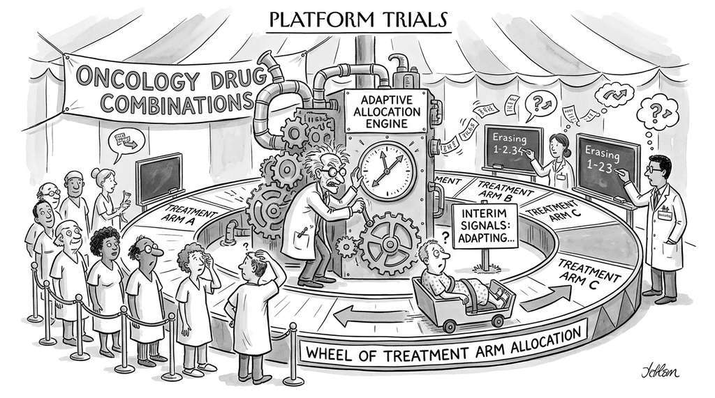
Novartis uses response-adaptive randomization (a contextual bandit variant) in their platform trials for oncology drug combinations. The system adjusts patient allocation across treatment arms after each cohort based on interim efficacy signals, funneling more patients toward promising combinations while maintaining statistical validity. Their RETHINK trial platform has reported roughly 30% fewer patients exposed to ineffective arms compared to equal-allocation designs, according to the company's published results, accelerating the identification of effective combination therapies.

4. Value of Information

Information-theoretic criteria tell us which experiment to run next, but not whether to run another experiment at all. The Value of Information (VOI) framework (Raiffa & Schlaifer, 1961) answers this stopping question by computing the expected improvement in decision quality from obtaining one more observation.

Suppose we must make a decision \(d \in \mathcal{D}\) (approve a drug, select a material, deploy a model) that yields utility \(u(d, \omega)\) depending on the unknown state \(\omega\). Our current best decision is:

with expected utility \(U^* = \max_d \mathbb{E}_\omega[u(d, \omega)]\). If we run experiment \(x\) and observe outcome \(y\), we can make a potentially better decision \(d^*_{x,y}\) using the updated posterior \(p(\omega \mid \mathcal{D} \cup \{(x,y)\})\). The expected value of sample information (EVSI) for experiment \(x\) is:

EVSI quantifies the expected gain in decision utility from running experiment \(x\). If \(\text{EVSI}(x) < \text{cost}(x)\) for all candidate experiments \(x\), we should stop experimenting: no experiment is worth its cost. This provides a principled stopping criterion that information-theoretic acquisition functions lack, and it connects directly to the stopping decision shown in Figure 46.3.

def compute_evsi(gp_model, X_pool, decision_threshold, cost_per_experiment,
                 n_mc=500, noise_std=0.1):
    """Compute Expected Value of Sample Information for each candidate.

    Decision: classify the function value at each point as above or
    below a threshold (e.g., "is this compound active?").

    Args:
        gp_model: fitted GaussianProcessRegressor
        X_pool: (n_pool, n_features) candidate experiments
        decision_threshold: threshold for the binary decision
        cost_per_experiment: cost of running one experiment
        n_mc: Monte Carlo samples for EVSI estimation

    Returns:
        evsi_scores: (n_pool,) expected value of information per point
        net_value: (n_pool,) EVSI minus cost (positive = worth running)
    """
    mu, std = gp_model.predict(X_pool, return_std=True)
    n_pool = len(X_pool)
    evsi_scores = np.zeros(n_pool)

    for i in range(n_pool):
        # Current decision: P(f(x) > threshold) based on current posterior
        p_above_current = 1.0 - _norm_cdf(
            (decision_threshold - mu[i]) / (std[i] + 1e-10)
        )
        current_utility = max(p_above_current, 1.0 - p_above_current)

        # Simulate outcomes and compute updated decisions
        y_samples = np.random.normal(mu[i], np.sqrt(std[i]**2 + noise_std**2), n_mc)
        updated_utilities = np.zeros(n_mc)

        for j, y_obs in enumerate(y_samples):
            # Bayesian update: posterior after observing y at x_i
            # For GP, the updated mean and variance have closed forms
            prior_var = std[i] ** 2
            obs_var = noise_std ** 2
            post_var = 1.0 / (1.0 / prior_var + 1.0 / obs_var)
            post_mean = post_var * (mu[i] / prior_var + y_obs / obs_var)
            post_std = np.sqrt(post_var)

            p_above_updated = 1.0 - _norm_cdf(
                (decision_threshold - post_mean) / (post_std + 1e-10)
            )
            updated_utilities[j] = max(p_above_updated, 1.0 - p_above_updated)

        evsi_scores[i] = updated_utilities.mean() - current_utility

    net_value = evsi_scores - cost_per_experiment
    return evsi_scores, net_value


def _norm_cdf(x):
    """Standard normal CDF via the error function."""
    from math import erf, sqrt
    return 0.5 * (1.0 + erf(x / sqrt(2.0)))

The VOI framework connects experiment design to decision-making in a way that pure information theory does not. Two experiments might provide equal information (same mutual information), but one might be more decision-relevant because it resolves uncertainty about a critical region of the parameter space. EVSI captures this by weighting information by its impact on the downstream decision. This perspective is central to the sequential decision problems in Chapter 55: Self-Driving Laboratories, where each experiment has a real dollar cost and the stopping decision directly affects the lab's budget.

5. Bayesian Optimal Experimental Design with PyMC

The theory of what to measure next and when to stop translates directly into a runnable Bayesian design loop in PyMC.

PyMC provides a natural framework for Bayesian experimental design by making the posterior computation explicit. We define a probabilistic model, compute the prior predictive distribution, then evaluate how much each candidate experiment would update the posterior.

import pymc as pm
import arviz as az

def bayesian_experiment_design(observed_data, candidate_experiments,
                                n_candidates_to_evaluate=20, seed=42):
    """Bayesian optimal design for a dose-response experiment.

    Model: y = E_max * x / (EC50 + x) + noise
    This is the Hill equation, a standard sigmoidal model that relates
    drug dose (x) to biological response (y) via two parameters: the
    maximum effect (E_max) and the dose producing half-maximal effect (EC50).

    Goal: select the dose x that maximally reduces posterior entropy of EC50.

    Args:
        observed_data: list of (dose, response) tuples
        candidate_experiments: (n_candidates,) array of candidate doses
        n_candidates_to_evaluate: how many candidates to score

    Returns:
        best_dose: the dose with highest expected information gain
        scores: dict mapping dose -> EIG score
    """
    doses = np.array([d[0] for d in observed_data])
    responses = np.array([d[1] for d in observed_data])

    scores = {}
    rng = np.random.default_rng(seed)
    eval_idx = rng.choice(
        len(candidate_experiments),
        size=min(n_candidates_to_evaluate, len(candidate_experiments)),
        replace=False
    )

    for idx in eval_idx:
        x_new = candidate_experiments[idx]

        # Fit current posterior
        with pm.Model() as model:
            E_max = pm.HalfNormal("E_max", sigma=2.0)
            EC50 = pm.LogNormal("EC50", mu=0.0, sigma=1.0)
            sigma = pm.HalfNormal("sigma", sigma=0.5)

            # Hill equation (dose-response)
            mu = E_max * doses / (EC50 + doses)
            pm.Normal("obs", mu=mu, sigma=sigma, observed=responses)

            trace = pm.sample(1000, tune=500, random_seed=seed,
                              progressbar=False)

        # Current posterior entropy of EC50
        ec50_samples = trace.posterior["EC50"].values.flatten()
        H_prior = _estimate_entropy(ec50_samples)

        # Simulate outcome at x_new and compute updated entropy
        H_posterior_samples = []
        for _ in range(50):
            # Sample EC50 and E_max from current posterior
            i = rng.integers(len(ec50_samples))
            ec50_s = ec50_samples[i]
            emax_s = trace.posterior["E_max"].values.flatten()[i]
            sigma_s = trace.posterior["sigma"].values.flatten()[i]

            # Simulate observation
            y_sim = emax_s * x_new / (ec50_s + x_new) + rng.normal(0, sigma_s)

            # Approximate updated posterior entropy (importance weighting:
            # reweight existing posterior samples by their likelihood under
            # the simulated observation, avoiding a full re-inference)
            log_likelihood = -(y_sim - emax_s * x_new / (ec50_samples + x_new))**2 / (2 * sigma_s**2)
            weights = np.exp(log_likelihood - log_likelihood.max())
            weights /= weights.sum()
            H_post = _weighted_entropy(ec50_samples, weights)
            H_posterior_samples.append(H_post)

        eig = H_prior - np.mean(H_posterior_samples)
        scores[x_new] = eig

    best_dose = max(scores, key=scores.get)
    return best_dose, scores


def _estimate_entropy(samples, n_bins=50):
    """Estimate entropy from samples using histogram method."""
    counts, _ = np.histogram(samples, bins=n_bins)
    probs = counts / counts.sum()
    probs = probs[probs > 0]
    return -np.sum(probs * np.log(probs))


def _weighted_entropy(samples, weights, n_bins=50):
    """Estimate entropy of a weighted sample distribution."""
    counts, bin_edges = np.histogram(samples, bins=n_bins, weights=weights)
    probs = counts / counts.sum()
    probs = probs[probs > 0]
    return -np.sum(probs * np.log(probs))

6. From Design to Discovery: Connecting the Pieces

Sequential design reuses the same GP surrogate as Bayesian optimization (Chapter 45), but targets global function learning rather than finding a maximum. The bandit algorithms extend the exploration/exploitation framework from Section 1.2 with Bayesian belief updates from Chapter 32, and the VOI stopping criterion complements the statistical stopping rules in Chapter 56.

In the Discovery Workbench, the sequential design module serves as the "brain" of the experiment loop: it receives observations from the data pipeline (Chapter 6), updates the surrogate model, computes acquisition scores for candidate experiments, selects the next batch, and dispatches it to the execution layer. The provenance of each selection (which acquisition function, what score, what alternatives were considered) is recorded in the experiment registry (Chapter 47).

Exercises

1. (Mathematical) Prove that BALD for a GP regression model with RBF kernel and known noise variance \(\sigma_n^2\) reduces to \(\frac{1}{2}\log(1 + \sigma^2(x)/\sigma_n^2)\). Start from the definition \(I(\theta; y \mid x, \mathcal{D}) = H[y \mid x, \mathcal{D}] - \mathbb{E}_\theta[H[y \mid x, \theta]]\) and use the fact that both terms involve Gaussian distributions.
2. (Coding) Implement a contextual Thompson Sampling bandit for a linear reward model (the Bayesian counterpart to LinUCB). Maintain a multivariate normal posterior over \(\theta\) and sample from it at each round. Compare to LinUCB on a synthetic problem with 5 arms and 10-dimensional context vectors. Which achieves lower regret?
3. (Analysis) Compute the EVSI for the dose-response model in Listing 46.13 at 20 candidate doses. Plot EVSI vs. dose and explain the shape of the curve. Why is EVSI highest near the EC50 and lowest at very low and very high doses?
4. (Research) The VOI stopping criterion requires a specified decision problem and utility function. Design a VOI-based stopping rule for an active learning classification task where the decision is "deploy the model" and the utility is test-set accuracy minus a per-query cost. Implement it and compare to a fixed-budget stopping rule on the two-moons dataset from Section 46.1.