7.1 SDLC as Iterative Hypothesis Testing

1. The Manufacturing Illusion

In 2005, the FBI scrapped the Virtual Case File project after spending over \$170 million, having discovered, years into development, that field agents needed something fundamentally different from what the specification described. Software engineering inherited its vocabulary from manufacturing. We talk about "building" software, "shipping" products, and running a "factory" of sprints. But nobody manufactures software. A developer writes each line of code exactly once (or should). No assembly line produces identical copies. Writing software means discovering what the program should be, one decision at a time.

Consider a concrete example. A team is asked to build a recommendation engine for a scientific paper discovery platform. At the start, they face cascading uncertainties:

• Requirements uncertainty: Do researchers want recommendations based on citation networks, content similarity, reading history, or some combination? How much novelty versus relevance do they prefer?
• Architecture uncertainty: Should the system use collaborative filtering, content-based filtering, a hybrid approach, or a large language model (LLM) for semantic matching?
• Implementation uncertainty: Which embedding model performs best on scientific text? What latency is acceptable? How should the system handle cold-start users, where "cold-start" refers to new users for whom the system has no prior interaction data to draw on?
• Value uncertainty: Will researchers actually use the recommendations? Will recommendations lead to better research outcomes, or just more reading?

Each of these uncertainties is a hypothesis waiting to be tested. The waterfall approach treats them as questions to be answered in sequence before writing code. The discovery approach treats them as experiments to be run as quickly as possible, with code as the experimental apparatus.

2. Formalizing SDLC as Search

When teams skip this formal mapping, they default to intuition about what to build next, and intuition scales poorly: the Standish Group's CHAOS reports consistently find that fewer than 35% of software projects succeed, with "incomplete requirements" and "lack of user involvement" topping every failure list. Making the search structure explicit is what turns those odds around.

The software development process maps directly onto the search framework from Section 1.1. The five-tuple \((S, A, T, f, C)\) for software discovery is:

• \(S\) (State space): the set of all possible software systems the team might build, including requirements documents, architecture diagrams, code, tests, and deployment configurations. Each state \(s \in S\) is a complete snapshot of the project.
• \(A\) (Actions): development activities such as writing a user story, implementing a feature, writing a test, refactoring, deploying to staging, running a user study, or merging a pull request.
• \(T\) (Transition function): \(T(s, a) \to s'\) describes how action \(a\) transforms project state \(s\) into a new state \(s'\). This function is stochastic because the outcome of writing code, running tests, or gathering user feedback is uncertain.
• \(f\) (Objective): a composite function measuring user satisfaction, system reliability, code maintainability, and development cost. In practice, \(f\) is partially observable and changes as the team learns more about what users actually need.
• \(C\) (Constraints): budget, timeline, team size, regulatory requirements, backward compatibility, and technical debt limits.

The key insight is that \(f\) is unknown at the start. The team does not fully know what a good outcome looks like until they have explored enough of the space to understand user needs. This makes software development a problem of search under uncertainty, precisely the setting where exploration strategies from Section 1.2 apply. In short: Software development is not a manufacturing problem with a known blueprint; it is a search problem with an unknown objective.

3. The Four Phases as Hypothesis Operations

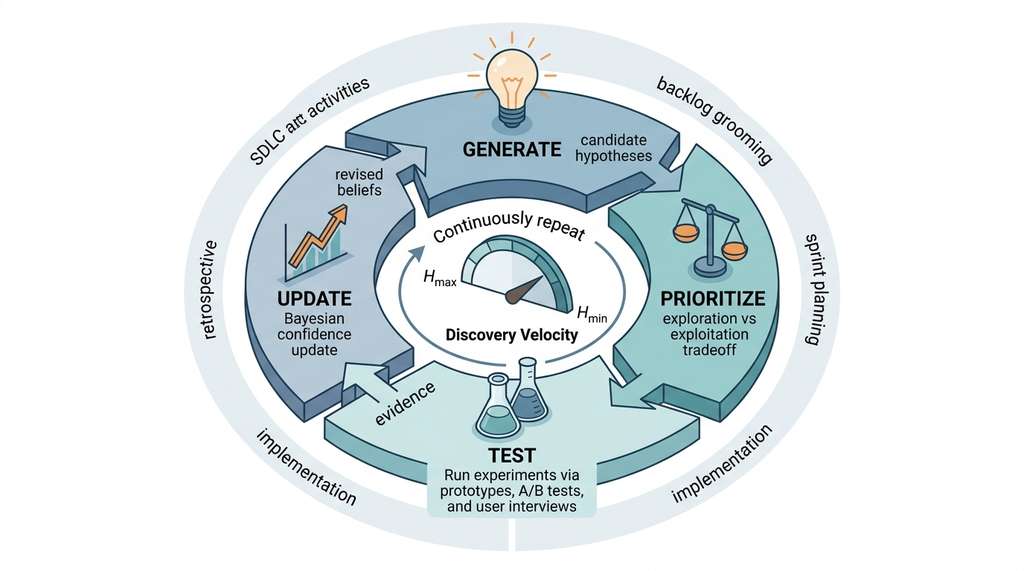
Every SDLC methodology, regardless of its specific practices, cycles through four fundamental operations on hypotheses. As Figure 7.1 illustrates, these four operations form a continuous loop, with each cycle's output feeding the next round of generation. We can formalize these using the language of Chapter 2:

Generation: producing candidate hypotheses about what to build and how. In agile, this happens during backlog grooming and sprint planning. In waterfall, it happens during requirements gathering. The quality of generation determines the breadth of the search.

Prioritization: selecting which hypotheses to test next. This is the exploration/exploitation trade-off from Section 1.2. Greedy prioritization (always build the feature with the highest expected value) exploits current knowledge but may miss better options. Exploratory prioritization (build the feature with the highest uncertainty) gathers information but delays value delivery.

Testing: running experiments to evaluate hypotheses. In software, experiments take many forms: unit tests, integration tests, A/B tests (controlled experiments that split users into groups to compare two variants of a feature), user interviews, prototype demos, canary deployments (where a new release is rolled out to a small subset of production servers before reaching all users), and production monitoring. Each reduces uncertainty about one or more hypotheses.

Updating: revising beliefs and plans based on experimental results. In Bayesian terms, we update our posterior distribution, the revised probability distribution over possible outcomes after observing new evidence, over the space of "good products" given the evidence gathered. In agile, this happens during retrospectives and backlog re-prioritization. Figure 7.1.1 illustrates SDLC hypothesis cycle with discovery velocity feedback loop.

The following formalization captures this cycle. Define a hypothesis \(h_i\) as a tuple \((claim_i, test_i, evidence_i, confidence_i)\) where \(claim_i\) is a falsifiable (that is, stated precisely enough to be proven wrong by a specific observation) statement about what to build, \(test_i\) is a procedure to evaluate the claim, \(evidence_i\) collects observations from running the test, and \(confidence_i \in [0, 1]\) is the team's posterior belief that the claim is correct.

from dataclasses import dataclass, field
from typing import Callable, Optional
import json
from datetime import datetime


@dataclass
class DevHypothesis:
    """A falsifiable hypothesis in a software development process.

    Each hypothesis represents an uncertain belief about what to build,
    how to build it, or whether it will deliver value. The confidence
    field tracks the team's evolving belief as evidence accumulates.
    """
    claim: str                           # Falsifiable statement
    category: str                        # "requirement", "architecture", "implementation", "value"
    test_procedure: str                  # How to test the claim
    success_criterion: str               # What counts as confirmation
    confidence: float = 0.5             # Prior belief, updated with evidence
    evidence: list = field(default_factory=list)
    status: str = "untested"            # "untested", "testing", "confirmed", "refuted"
    created_at: str = field(default_factory=lambda: datetime.now().isoformat())

    def update_confidence(self, observation: str, confirms: bool,
                          strength: float = 0.1) -> float:
        """Bayesian-style confidence update given new evidence.

        Uses a simplified update rule: confidence moves toward 1.0 if
        the observation confirms the hypothesis, toward 0.0 if it refutes.
        The strength parameter controls the magnitude of the update.
        """
        if confirms:
            self.confidence = self.confidence + strength * (1.0 - self.confidence)
        else:
            self.confidence = self.confidence - strength * self.confidence

        self.evidence.append({
            "observation": observation,
            "confirms": confirms,
            "strength": strength,
            "timestamp": datetime.now().isoformat(),
            "confidence_after": round(self.confidence, 4)
        })

        # Update status based on accumulated evidence
        if self.confidence > 0.9:
            self.status = "confirmed"
        elif self.confidence < 0.1:
            self.status = "refuted"
        else:
            self.status = "testing"

        return self.confidence

    def to_user_story(self) -> str:
        """Convert a confirmed requirement hypothesis to a user story."""
        if self.category != "requirement":
            raise ValueError("Only requirement hypotheses become user stories")
        return f"As a user, I want {self.claim} so that {self.success_criterion}"


# Example: hypotheses for a paper recommendation system
hypotheses = [
    DevHypothesis(
        claim="Researchers prefer citation-based recommendations over content similarity",
        category="requirement",
        test_procedure="A/B test with 50 users comparing citation-graph vs. embedding similarity",
        success_criterion="Citation-based click-through rate (CTR) exceeds content-based CTR by >10%",
        confidence=0.6  # Slight prior toward citation-based
    ),
    DevHypothesis(
        claim="SPECTER2 embeddings outperform TF-IDF for scientific paper similarity",
        category="implementation",
        test_procedure="Offline evaluation on RELISH benchmark dataset",
        success_criterion="SPECTER2 achieves >0.85 normalized Discounted Cumulative Gain (nDCG) @10 vs TF-IDF baseline",
        confidence=0.7  # Strong prior based on published results
    ),
    DevHypothesis(
        claim="Users will engage with recommendations if latency is under 200ms",
        category="value",
        test_procedure="Deploy with latency monitoring and track engagement rate",
        success_criterion="Engagement rate >15% when p95 latency < 200ms",
        confidence=0.5  # Genuine uncertainty
    ),
]

# Simulate evidence arriving from experiments
hypotheses[0].update_confidence("Pilot users clicked 2x more on citation recs", True, 0.2)
hypotheses[0].update_confidence("Power users preferred content recs for cross-field", False, 0.15)

for h in hypotheses:
    print(f"[{h.status:>10}] {h.confidence:.2f}  {h.claim[:60]}...")

4. Discovery Velocity

If software development is discovery, we need a metric for how fast a team is discovering. Lines of code per day and story points per sprint measure output, not learning. A team that ships ten features nobody wants has high output velocity but zero discovery velocity.

We define discovery velocity \(v_d\) as the rate of uncertainty reduction per unit time:

Discovery velocity measures how quickly a team converts unknowns into validated decisions, expressed in bits of resolved uncertainty per unit time. It matters because traditional productivity metrics (lines of code, features shipped) reward output regardless of whether that output addresses the right problem, while discovery velocity directly captures the team's rate of learning. The mechanism is straightforward: each tested hypothesis either confirms or refutes a belief, sharpening the team's probability distribution over possible products and reducing its Shannon entropy, the information-theoretic measure of uncertainty in a probability distribution (Shannon, 1948). Use discovery velocity when the primary risk is building the wrong thing (most new products and features); fall back to throughput metrics only for well-understood maintenance work where requirements are stable and the search space is already narrow.

where \(H(S_t)\) is the entropy of the team's belief distribution over "what is the right product to build" at time \(t\). When \(H\) is high, the team is uncertain; as hypotheses are tested and beliefs sharpen, \(H\) decreases. A team with high discovery velocity resolves uncertainty quickly, converging on the right product faster.

In practice, we approximate \(H\) using the set of active hypotheses:

where \(c_i\) is the confidence in hypothesis \(i\) and \(n\) is the number of active hypotheses. Note that the logarithm is base 2 so that entropy is measured in bits, matching the code in Listing 7.2. Each term reaches its maximum of 1 bit when \(c_i = 0.5\) (maximum uncertainty) and drops to zero when \(c_i\) approaches 0 or 1 (resolved).

import numpy as np
from typing import List


def compute_entropy(hypotheses: List[DevHypothesis]) -> float:
    """Compute the total uncertainty across all active hypotheses.

    Uses binary entropy for each hypothesis: maximum at confidence = 0.5,
    zero at confidence = 0 or 1. The sum gives total team uncertainty.
    """
    total = 0.0
    for h in hypotheses:
        c = np.clip(h.confidence, 1e-10, 1 - 1e-10)  # Avoid log(0)
        total += -(c * np.log2(c) + (1 - c) * np.log2(1 - c))
    return total


def discovery_velocity(hypotheses: List[DevHypothesis],
                       entropy_before: float,
                       time_elapsed_days: float) -> float:
    """Compute discovery velocity as bits of uncertainty resolved per day."""
    entropy_after = compute_entropy(hypotheses)
    return (entropy_before - entropy_after) / max(time_elapsed_days, 1e-6)


# Measure discovery velocity for our recommendation system team
entropy_t0 = compute_entropy(hypotheses)
print(f"Initial entropy: {entropy_t0:.3f} bits")

# After one sprint (2 weeks), some hypotheses have been tested
hypotheses[1].update_confidence("SPECTER2 nDCG@10 = 0.91 on RELISH", True, 0.25)
hypotheses[2].update_confidence("Prototype p95 latency = 150ms, engagement = 18%", True, 0.3)

entropy_t1 = compute_entropy(hypotheses)
v_d = discovery_velocity(hypotheses, entropy_t0, time_elapsed_days=14)
print(f"Entropy after sprint: {entropy_t1:.3f} bits")
print(f"Discovery velocity: {v_d:.4f} bits/day")

5. The Expected Regret of Greedy Development

Discovery velocity tells us how fast a team is learning, but it does not yet explain what happens when a team skips exploration altogether and bets everything on the first plausible idea.

Why not just build the first idea that seems good? The answer lies in the regret analysis from Section 1.2. Greedy development, where the team commits fully to the highest-expected-value feature without exploring alternatives, incurs expected regret that grows with the uncertainty in the environment.

Define the expected regret of greedy development over \(T\) sprints as:

where \(a^*_t\) is the optimal action at time \(t\) (knowable only in hindsight) and \(a_t^{\text{greedy}}\) is the action chosen by the greedy strategy. The key result from bandit theory, a branch of decision theory that studies how to allocate a fixed budget of attempts among competing options with unknown payoffs, is that greedy regret grows linearly with \(T\) when the environment is uncertain, while exploratory strategies (UCB, Thompson Sampling) achieve regret that grows only as \(O(\log T)\), scaling logarithmically rather than linearly with the number of rounds (Auer et al., 2002).

import numpy as np
import matplotlib.pyplot as plt


def simulate_dev_strategies(n_sprints: int = 50,
                            n_features: int = 10,
                            seed: int = 42) -> dict:
    """Simulate greedy vs. exploratory development over multiple sprints.

    Each 'feature' has a true value drawn from a distribution unknown to
    the team. The greedy strategy always picks the feature with the highest
    estimated value. The exploratory (UCB-style) strategy balances estimated
    value with uncertainty, exploring less-known features.

    Returns cumulative regret for each strategy.
    """
    rng = np.random.default_rng(seed)

    # True feature values (unknown to the team)
    true_values = rng.beta(2, 5, size=n_features)  # Skewed: most features mediocre
    true_values[rng.choice(n_features)] = 0.9       # One great feature, hidden

    # Team's estimates and observation counts
    estimates = np.full(n_features, 0.5)  # Uniform prior
    counts = np.zeros(n_features)

    greedy_regret = []
    ucb_regret = []
    optimal_value = true_values.max()

    greedy_total = 0.0
    ucb_total = 0.0

    ucb_estimates = estimates.copy()
    ucb_counts = np.zeros(n_features)

    for t in range(1, n_sprints + 1):
        # Greedy: pick the feature with highest current estimate
        greedy_choice = np.argmax(estimates)
        greedy_reward = true_values[greedy_choice] + rng.normal(0, 0.1)
        counts[greedy_choice] += 1
        # Update estimate (running average)
        estimates[greedy_choice] += (greedy_reward - estimates[greedy_choice]) / counts[greedy_choice]
        greedy_total += optimal_value - true_values[greedy_choice]
        greedy_regret.append(greedy_total)

        # UCB: balance exploitation and exploration
        ucb_scores = np.where(
            ucb_counts > 0,
            ucb_estimates + np.sqrt(2 * np.log(t) / ucb_counts),
            float('inf')  # Explore untried features first
        )
        ucb_choice = np.argmax(ucb_scores)
        ucb_reward = true_values[ucb_choice] + rng.normal(0, 0.1)
        ucb_counts[ucb_choice] += 1
        ucb_estimates[ucb_choice] += (ucb_reward - ucb_estimates[ucb_choice]) / ucb_counts[ucb_choice]
        ucb_total += optimal_value - true_values[ucb_choice]
        ucb_regret.append(ucb_total)

    return {
        "greedy_regret": greedy_regret,
        "ucb_regret": ucb_regret,
        "true_values": true_values,
        "sprints": list(range(1, n_sprints + 1))
    }


results = simulate_dev_strategies()

# The greedy strategy accumulates roughly linear regret,
# while UCB's regret flattens as it discovers the best feature
print(f"Greedy total regret after 50 sprints: {results['greedy_regret'][-1]:.2f}")
print(f"UCB total regret after 50 sprints:    {results['ucb_regret'][-1]:.2f}")
print(f"Regret ratio (greedy/UCB):            {results['greedy_regret'][-1] / max(results['ucb_regret'][-1], 0.01):.1f}x")

6. SDLC Models as Exploration Strategies

The regret analysis above treats exploration as a single knob to turn up or down, but real development teams encode their exploration choices into a methodology, each with its own feedback rhythm and risk profile.

Different SDLC methodologies correspond to different strategies for navigating the search space. We can characterize each by its exploration/exploitation ratio and the feedback loop length (how quickly hypotheses are tested).

Methodology Profiles

Waterfall is a pure exploitation strategy: commit to a single path through the search space (the specification) and follow it to completion. Feedback arrives only at deployment. In bandit terms, waterfall is equivalent to pulling the same arm for all \(T\) rounds without observing rewards. This works well when uncertainty is very low (the team has built similar systems before) but incurs catastrophic regret when assumptions are wrong.

Agile/Scrum introduces periodic exploration through sprint cycles. Each sprint is a mini-experiment: the team builds a small increment, gathers feedback, and adjusts. The sprint length (typically 1 to 4 weeks) determines the feedback loop latency. Shorter sprints mean faster hypothesis testing, but each individual experiment has less power (less code built, fewer features to evaluate).

Lean Startup pushes exploration further by minimizing the cost of each experiment. The minimum viable product (MVP) is the smallest possible test of the most critical hypothesis. Build-measure-learn cycles can be as short as hours or days. In bandit terms, lean development reduces the cost per arm pull, enabling more exploration within the same budget. Under the parameters in Listing 7.4, a Lean/MVP team can test roughly 60 hypotheses per quarter; a Waterfall team, following the same model, tests fewer than one.

Design Thinking adds a distinct generation phase (ideation) before testing. While agile and lean tend to test hypotheses sequentially, design thinking encourages generating a broad set of candidates before selecting any for implementation. This corresponds to a higher exploration budget in the early phases, trading short-term progress for a better initial survey of the search space.

from dataclasses import dataclass


@dataclass
class SDLCStrategy:
    """Characterize an SDLC methodology as a search strategy."""
    name: str
    exploration_ratio: float      # Fraction of effort spent exploring alternatives
    feedback_loop_days: float     # Average time to test one hypothesis
    cost_per_experiment: float    # Relative cost of each experiment (1.0 = full feature)
    parallelism: int              # Number of hypotheses tested simultaneously

    @property
    def hypotheses_per_quarter(self) -> float:
        """Estimate how many hypotheses a team can test in 90 days."""
        sequential = 90 / self.feedback_loop_days
        return sequential * self.parallelism

    @property
    def regret_profile(self) -> str:
        if self.exploration_ratio < 0.1:
            return "Linear (high risk of locking onto suboptimal path)"
        elif self.exploration_ratio < 0.3:
            return "Sublinear (moderate exploration mitigates lock-in)"
        else:
            return "Logarithmic (broad exploration, slower initial delivery)"


strategies = [
    SDLCStrategy("Waterfall",      0.05,  180,  1.0,   1),
    SDLCStrategy("Scrum (2-week)", 0.20,   14,  0.3,   1),
    SDLCStrategy("Lean/MVP",       0.35,    3,  0.05,  2),
    SDLCStrategy("Design Thinking",0.50,    7,  0.1,   3),
]

print(f"{'Strategy':<20} {'Explore%':>8} {'Loop(d)':>8} "
      f"{'Hyp/Qtr':>8}  {'Regret Profile'}")
print("-" * 85)
for s in strategies:
    print(f"{s.name:<20} {s.exploration_ratio:>7.0%} {s.feedback_loop_days:>8.0f} "
          f"{s.hypotheses_per_quarter:>8.0f}  {s.regret_profile}")

Exercises

1. (Conceptual) Take a software project you have worked on (or are currently working on). Identify three hypotheses that the team held implicitly. For each, write the claim, test procedure, and success criterion in the DevHypothesis format. Were any of these hypotheses tested before full implementation? What would have changed if they had been?
2. (Coding) Extend the simulate_dev_strategies function to include a Thompson Sampling strategy alongside greedy and UCB. Compare the regret curves of all three over 100 sprints. Which strategy discovers the best feature fastest? At what sprint count does each strategy's regret curve begin to flatten?
3. (Analysis) Compute the discovery velocity for two hypothetical teams: Team A runs 2-week sprints and resolves one hypothesis per sprint; Team B runs 1-week sprints but resolves only 0.4 hypotheses per sprint (due to lower experiment power). Which team has higher discovery velocity? Under what conditions does Team B's shorter cycle outweigh its lower per-cycle resolution rate?