7.2 Engineering Discovery and AI

1. The Cost Structure of Software Discovery

Teams that adopt AI coding tools without understanding which cost they are reducing often speed up the wrong bottleneck, shipping features faster while learning nothing new about what to build. The cost model below makes the bottleneck explicit, so you can target AI where it actually multiplies discovery.

In the framework of Section 7.1, each hypothesis test has four cost components: generation cost \(c_g\) (time to formulate the hypothesis and plan the experiment), implementation cost \(c_i\) (time to write the experimental code), execution cost \(c_e\) (time to run tests, deploy, and collect data), and analysis cost \(c_a\) (time to interpret results and update beliefs). The total cost per hypothesis is:

And the discovery velocity from Section 7.1 becomes:

where \(\Delta H\) is the total entropy reduction (bits of uncertainty resolved) across all tests and \(n\) is the number of hypotheses tested. AI affects each cost component differently, and understanding these effects is essential for designing effective AI-augmented development workflows. In short: the team that knows which cost dominates its discovery loop is the one that benefits most from AI; the team that does not just builds the wrong product faster.

Discovery velocity measures how fast a team reduces its uncertainty about what to build, in bits of resolved entropy (the information-theoretic measure of remaining uncertainty: when many outcomes are still plausible, entropy is high; when the team has converged on a clear direction, entropy is low) per unit of time (a sprint or calendar day). Two teams with identical coding speed can have vastly different product outcomes. The team that resolves uncertainty faster converges on the right product sooner, avoiding weeks or months of building the wrong thing. The mechanism: each hypothesis test confirms or refutes an assumption, collapsing a branch of the decision tree and lowering entropy. Use discovery velocity rather than raw throughput (features shipped, lines of code) when the primary risk is building the wrong product. Use throughput metrics when the product direction is validated and the bottleneck is execution.

How AI Affects Each Cost Component

Generation cost \(c_g\): AI reduces this through brainstorming assistance. A large language model (LLM) can rapidly generate alternative hypotheses, suggest edge cases, and identify assumptions the team has not considered. A prompt like "Given a paper recommendation system, what are ten hypotheses about user behavior that would change the architecture?" produces candidates in seconds that might take a team meeting to surface.

Implementation cost \(c_i\): this is where AI has the most dramatic effect. Code generation tools (GitHub Copilot, Claude Code, Cursor) can produce working prototypes from natural language descriptions, reducing \(c_i\) by an estimated 3x to 10x for well-specified tasks, though measured gains vary with task complexity and developer experience. (A 5x drop in implementation cost means a team can afford five prototype experiments for the price of one, turning "pick your best guess" into "test them all.") This is the core mechanism that shifts the optimal exploration strategy.

Execution cost \(c_e\): AI assists through automated test generation, intelligent continuous integration/continuous deployment (CI/CD) pipelines, and anomaly detection in production metrics. These reduce the latency between "code is written" and "hypothesis is evaluated."

Analysis cost \(c_a\): AI helps interpret results through automated log analysis, metric summarization, and pattern detection. When a deployment produces unexpected behavior, an AI assistant can scan logs and surface the relevant signals faster than manual investigation.

from dataclasses import dataclass
import numpy as np


@dataclass
class DiscoveryCostModel:
    """Model the cost structure of hypothesis testing with and without AI.

    All costs are in developer-hours per hypothesis.
    """
    generation_hours: float
    implementation_hours: float
    execution_hours: float
    analysis_hours: float

    @property
    def total_hours(self) -> float:
        return (self.generation_hours + self.implementation_hours +
                self.execution_hours + self.analysis_hours)

    def hypotheses_per_sprint(self, sprint_hours: float = 80) -> float:
        """How many hypotheses can a developer test per sprint (2 weeks)?"""
        return sprint_hours / self.total_hours


# Traditional development costs (experienced team, no AI)
traditional = DiscoveryCostModel(
    generation_hours=4.0,     # Requirements discussion, planning
    implementation_hours=24.0, # Writing code, debugging, reviewing
    execution_hours=8.0,      # Running tests, deploying, waiting
    analysis_hours=4.0        # Analyzing results, writing up findings
)

# AI-assisted development costs
ai_assisted = DiscoveryCostModel(
    generation_hours=1.0,     # LLM brainstorming, rapid ideation
    implementation_hours=4.0,  # AI code generation + human review
    execution_hours=4.0,      # Automated test generation, faster CI
    analysis_hours=2.0        # AI-assisted log analysis
)

print(f"{'Metric':<30} {'Traditional':>12} {'AI-Assisted':>12} {'Speedup':>8}")
print("-" * 65)
print(f"{'Total hours/hypothesis':<30} {traditional.total_hours:>12.1f} "
      f"{ai_assisted.total_hours:>12.1f} {traditional.total_hours/ai_assisted.total_hours:>7.1f}x")
print(f"{'Hypotheses/sprint':<30} {traditional.hypotheses_per_sprint():>12.1f} "
      f"{ai_assisted.hypotheses_per_sprint():>12.1f} "
      f"{ai_assisted.hypotheses_per_sprint()/traditional.hypotheses_per_sprint():>7.1f}x")

# The implication for discovery velocity
# If each hypothesis resolves ~0.5 bits of entropy on average:
bits_per_hyp = 0.5
sprint_days = 14
trad_velocity = (traditional.hypotheses_per_sprint() * bits_per_hyp) / sprint_days
ai_velocity = (ai_assisted.hypotheses_per_sprint() * bits_per_hyp) / sprint_days
print(f"\n{'Discovery velocity (bits/day)':<30} {trad_velocity:>12.3f} "
      f"{ai_velocity:>12.3f} {ai_velocity/trad_velocity:>7.1f}x")

2. Agile, Lean, and Design Thinking as Discovery Strategies

Section 7.1 characterized SDLC methodologies by their exploration ratio and feedback loop length. AI changes the dynamics of each.

Agile with AI: the sprint remains the basic experiment cycle, but AI compresses what fits within a sprint. A sprint that previously tested one hypothesis now tests three or four. The risk is that teams confuse increased output (more features) with increased discovery (more learning). The discipline of the hypothesis framework is essential: every sprint should begin with explicit hypotheses and end with explicit evidence, regardless of how many features were shipped.

Lean with AI: the minimum viable product becomes even more minimal. When an AI assistant can generate a functional prototype from a natural language specification in under an hour, the "minimum" in MVP drops to a conversation with a language model followed by a live demo. This is the essence of vibe coding, covered in depth in Chapter 9. The build-measure-learn cycle compresses from days to hours.

Design thinking with AI: the ideation phase benefits enormously from AI's ability to generate diverse alternatives. Instead of a team brainstorm producing 10 ideas, an AI-augmented session can produce 50 or more candidates, drawn from patterns across millions of prior solutions. The challenge shifts from "generating enough ideas" to "filtering and prioritizing the best ones," a task that itself benefits from systematic evaluation frameworks.

To quantify how these cheaper exploration cycles shift the balance between trying new approaches and committing to known ones, we can simulate the explore/exploit trade-off directly.

from dataclasses import dataclass
from typing import List, Tuple
import numpy as np


@dataclass
class ExplorationSimulator:
    """Simulate how AI changes the exploration/exploitation balance.

    Models a team choosing between 'build next feature' (exploit)
    and 'prototype alternative approach' (explore), with AI reducing
    the cost of exploration.
    """
    n_options: int = 8              # Number of possible approaches
    true_values: np.ndarray = None  # Hidden quality of each approach
    noise_std: float = 0.15         # Observation noise

    def __post_init__(self):
        if self.true_values is None:
            rng = np.random.default_rng(123)
            # Most options are mediocre; one is excellent
            self.true_values = rng.uniform(0.2, 0.6, self.n_options)
            self.true_values[5] = 0.95  # The hidden gem

    def run_strategy(self, explore_ratio: float, budget: int,
                     cost_per_explore: float = 1.0,
                     seed: int = 0) -> Tuple[float, List[float]]:
        """Run an explore-then-exploit strategy.

        Spends explore_ratio of budget on exploration (trying different
        options), then exploits the best-found option for the remainder.
        cost_per_explore < 1.0 models AI making exploration cheaper.
        """
        rng = np.random.default_rng(seed)
        explore_budget = int(budget * explore_ratio / cost_per_explore)
        exploit_budget = budget - int(budget * explore_ratio)

        # Exploration phase: try options and observe noisy rewards
        observations = {}
        for i in range(explore_budget):
            option = i % self.n_options
            reward = self.true_values[option] + rng.normal(0, self.noise_std)
            observations.setdefault(option, []).append(reward)

        # Pick the best based on observations
        if observations:
            avg_rewards = {k: np.mean(v) for k, v in observations.items()}
            best_option = max(avg_rewards, key=avg_rewards.get)
        else:
            best_option = 0  # Default if no exploration

        # Exploitation phase: collect rewards from best option
        total_reward = sum(
            self.true_values[best_option] + rng.normal(0, self.noise_std)
            for _ in range(exploit_budget)
        )

        # Also count exploration rewards
        for rewards in observations.values():
            total_reward += sum(rewards)

        return total_reward, list(observations.keys())


sim = ExplorationSimulator()

# Compare strategies at different exploration ratios and AI cost reductions
configs = [
    ("Traditional, 10% explore",  0.10, 1.0),
    ("Traditional, 30% explore",  0.30, 1.0),
    ("AI-assisted, 10% explore",  0.10, 0.2),  # AI makes exploring 5x cheaper
    ("AI-assisted, 30% explore",  0.30, 0.2),
    ("AI-assisted, 50% explore",  0.50, 0.2),
]

budget = 100
print(f"{'Strategy':<30} {'Reward':>8} {'Options Tried':>14} {'Found Best?':>12}")
print("-" * 68)
for name, ratio, cost in configs:
    reward, explored = sim.run_strategy(ratio, budget, cost, seed=42)
    found_best = 5 in explored  # Option 5 is the hidden gem
    print(f"{name:<30} {reward:>8.1f} {len(set(explored)):>14} "
          f"{'Yes' if found_best else 'No':>12}")

3. AI as a Discovery Accelerator Across SDLC Phases

AI tools affect each phase of the hypothesis-driven SDLC from Section 7.1 differently.

Hypothesis generation: LLMs excel at generating diverse alternatives. Given a product description, an LLM can propose user personas, identify unstated assumptions, generate competing architectural approaches, and enumerate failure modes. The key is prompt engineering for divergence: asking the model to generate ideas that are maximally different from each other, not variations on a theme. Chapter 10 develops this technique further.

"""
Prompt template for hypothesis generation using an LLM.

This is a structured prompt that elicits diverse, falsifiable hypotheses
about a software product. The key elements are:
1. Context about the product domain
2. Request for DIVERSE (not similar) hypotheses
3. Requirement for falsifiability and testability
4. Structured output format matching our DevHypothesis class
"""

HYPOTHESIS_GENERATION_PROMPT = """
You are helping a software team identify the key uncertainties in their product.

Product: {product_description}
Target users: {target_users}
Known constraints: {constraints}

Generate {n_hypotheses} DIVERSE hypotheses about this product. Each hypothesis
should represent a genuinely different uncertainty (not variations on the same
theme). Cover these categories:
- User behavior hypotheses (what users actually want)
- Technical hypotheses (which approach will work best)
- Value hypotheses (whether the product will deliver its intended value)
- Integration hypotheses (how the product fits into existing workflows)

For each hypothesis, provide:
1. CLAIM: A falsifiable statement (can be proven wrong)
2. CATEGORY: requirement | architecture | implementation | value
3. TEST: How to test this in under one sprint
4. SUCCESS_CRITERION: A measurable threshold for confirmation
5. PRIOR_CONFIDENCE: Your estimated probability (0.0 to 1.0) with reasoning

Format each as JSON matching this schema:
{{"claim": str, "category": str, "test_procedure": str,
  "success_criterion": str, "confidence": float}}
"""


def generate_hypotheses(product_desc: str, target_users: str,
                        constraints: str, n: int = 8) -> str:
    """Format the hypothesis generation prompt.

    In production, this would be sent to an LLM API. Here we show
    the prompt construction. See Chapter 10 for the full LLM
    integration pattern.
    """
    return HYPOTHESIS_GENERATION_PROMPT.format(
        product_description=product_desc,
        target_users=target_users,
        constraints=constraints,
        n_hypotheses=n
    )


# Example usage for our paper recommendation system
prompt = generate_hypotheses(
    product_desc="AI-powered scientific paper recommendation engine",
    target_users="Graduate students and postdoctoral researchers",
    constraints="Must integrate with existing reference managers; "
                "latency under 500ms; privacy-preserving (no tracking)",
    n=6
)
print(prompt[:500] + "...")

Hypothesis prioritization: given a portfolio of hypotheses, AI can assist with prioritization by estimating the information value of each test. The concept of value of information from decision theory tells us that the most valuable hypothesis to test is the one whose outcome would most change our development plan. An LLM can help estimate this by reasoning about dependencies between hypotheses.

from typing import List, Dict
import json


def prioritize_hypotheses(hypotheses: list,
                          dependencies: Dict[str, List[str]]) -> list:
    """Prioritize hypotheses by estimated information value.

    Information value is higher when:
    1. The hypothesis is highly uncertain (confidence near 0.5)
    2. Many other hypotheses depend on it (high fan-out)
    3. The cost of testing is low relative to the information gained

    This is a simplified version; Section 46 covers full
    expected information gain computation.
    """
    scored = []
    for h in hypotheses:
        # Uncertainty: maximum at confidence = 0.5
        uncertainty = 1.0 - abs(2 * h.confidence - 1.0)

        # Fan-out: how many other hypotheses depend on this one
        dependents = len(dependencies.get(h.claim[:30], []))
        fan_out_score = 1.0 + 0.3 * dependents

        # Combined score (higher = test first)
        info_value = uncertainty * fan_out_score
        scored.append((info_value, h))

    # Sort by information value, descending
    scored.sort(key=lambda x: x[0], reverse=True)
    return scored


# Using our earlier hypotheses from Section 7.1
from section_7_1_examples import hypotheses  # Conceptual import

dependencies = {
    "Researchers prefer citat": ["SPECTER2 embeddings out"],
    # The embedding choice depends on whether we use content similarity
}

# In practice: prioritized = prioritize_hypotheses(hypotheses, dependencies)
# The hypothesis with highest uncertainty AND most dependents goes first

Automated testing as falsification: in the scientific method, a hypothesis gains credibility not by being "verified" but by surviving attempts at falsification. Software testing is precisely this: each test case is an attempt to falsify the claim that the code works correctly. AI-generated tests are particularly valuable here because they explore edge cases that human developers overlook. Chapter 18 covers AI-assisted testing extensively.

Once code survives its test suite, the experiment moves from the controlled environment of the development machine to the unpredictable conditions of production, where real user behavior becomes the ultimate arbiter.

Belief updating with production data: once deployed, code faces real users, and production metrics become ongoing experiments. Feature flags (configuration toggles that enable or disable a feature for specific user segments without redeploying code), A/B tests, and canary deployments gather evidence about hypotheses under real conditions. AI monitors metric dashboards, detects anomalies, and summarizes results. These tasks grow infeasible for humans as systems scale. This connects directly to the MLOps and observability practices in Chapter 22.

4. The Discovery Amplification Effect

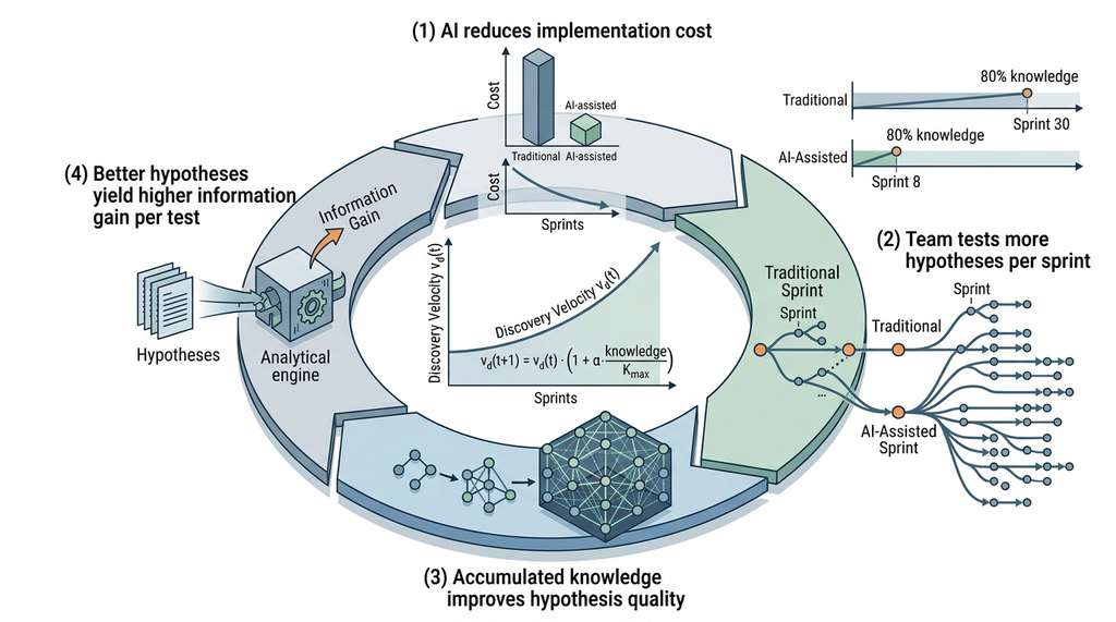
AI does not just make individual hypothesis tests cheaper; it creates a compounding effect called discovery amplification. More hypotheses per sprint accelerates knowledge accumulation, which sharpens future hypothesis generation and yields better-targeted experiments, compounding the advantage over time. Formally:

where \(\alpha\) is the amplification coefficient, a tunable parameter capturing how strongly the team's accumulated knowledge improves the quality of its future hypotheses (typical values range from 0.3 for siloed teams to 0.7 for teams with strong knowledge-sharing practices) and \(K_{\max}\) is the total knowledge needed to build the product. This positive feedback loop means that teams that adopt AI-assisted discovery early gain a compounding advantage over time. Figure 7.2 illustrates this cycle. Figure 7.2.1 illustrates Discovery amplification feedback loop with AI cost reduction.

However, amplification has limits. As the team converges on the right product, the marginal value of each additional hypothesis test decreases (diminishing returns on exploration). The optimal strategy transitions from broad exploration to focused exploitation as uncertainty decreases, exactly the UCB dynamic from Section 1.2.

Putting these pieces together, AI-assisted development achieves higher discovery velocity than traditional approaches when three conditions hold: (1) implementation cost \(c_i\) is the dominant term in the team's cost equation, so that reducing it yields a meaningful drop in \(c_{\text{total}}\); (2) the team increases its exploration ratio to match the cheaper cost of prototyping, rather than simply shipping the same number of features faster; and (3) the problem space contains enough viable alternatives that broader search is likely to surface a meaningfully better option. When the bottleneck is instead analysis (\(c_a\)) or execution (\(c_e\)), or when the product direction is already well understood and the remaining work is pure execution, the amplification effect is weak and AI's primary benefit reduces to a straightforward speedup.

import numpy as np


def simulate_amplification(n_sprints: int = 30,
                           ai_speedup: float = 4.0,
                           alpha: float = 0.5,
                           seed: int = 42) -> dict:
    """Simulate the discovery amplification effect.

    Compare a traditional team (constant discovery velocity) with an
    AI-assisted team (accelerating discovery due to knowledge compounding).
    """
    rng = np.random.default_rng(seed)

    # Initial knowledge and target
    k_max = 100.0  # Total "knowledge units" to build the product
    base_rate = 2.0  # Knowledge units per sprint (traditional)

    # Traditional: constant rate
    trad_knowledge = []
    k = 0.0
    for t in range(n_sprints):
        k += base_rate + rng.normal(0, 0.3)
        k = min(k, k_max)
        trad_knowledge.append(k)

    # AI-assisted: amplified rate
    ai_knowledge = []
    k = 0.0
    rate = base_rate * ai_speedup  # Start faster
    for t in range(n_sprints):
        # Rate increases as knowledge accumulates (amplification)
        effective_rate = rate * (1 + alpha * k / k_max)
        # But diminishing returns as we approach k_max
        remaining_fraction = (k_max - k) / k_max
        k += effective_rate * remaining_fraction + rng.normal(0, 0.3)
        k = min(k, k_max)
        ai_knowledge.append(k)

    return {
        "sprints": list(range(1, n_sprints + 1)),
        "traditional": trad_knowledge,
        "ai_assisted": ai_knowledge,
    }


results = simulate_amplification()

# Find sprint where each team reaches 80% knowledge
trad_80 = next(i for i, k in enumerate(results["traditional"]) if k >= 80)
ai_80 = next(i for i, k in enumerate(results["ai_assisted"]) if k >= 80)

print(f"Sprints to reach 80% product knowledge:")
print(f"  Traditional: sprint {trad_80 + 1}")
print(f"  AI-assisted: sprint {ai_80 + 1}")
print(f"  Time savings: {trad_80 - ai_80} sprints ({(trad_80 - ai_80) * 2} weeks)")

5. Measuring AI's Impact on Development Discovery

The following metrics evaluate whether AI tools actually improve a team's discovery process, not just its coding speed.

from dataclasses import dataclass, field
from typing import List
from datetime import datetime, timedelta


@dataclass
class SprintMetrics:
    """Metrics for evaluating discovery effectiveness in a sprint."""
    sprint_id: int
    hypotheses_tested: int          # Number of hypotheses evaluated
    hypotheses_resolved: int        # Confirmed or refuted (not still testing)
    entropy_start: float            # Team uncertainty at sprint start
    entropy_end: float              # Team uncertainty at sprint end
    features_shipped: int           # Features deployed to production
    experiments_run: int            # A/B tests, prototypes, user interviews
    pivot_decisions: int            # Times the team changed direction based on evidence
    wasted_effort_hours: float      # Hours spent on subsequently-refuted hypotheses

    @property
    def discovery_velocity(self) -> float:
        """Bits of uncertainty resolved per sprint."""
        return self.entropy_start - self.entropy_end

    @property
    def resolution_rate(self) -> float:
        """Fraction of tested hypotheses that reached a clear conclusion."""
        if self.hypotheses_tested == 0:
            return 0.0
        return self.hypotheses_resolved / self.hypotheses_tested

    @property
    def waste_ratio(self) -> float:
        """Fraction of effort spent on dead ends (lower is better)."""
        total_hours = 80  # Approximate sprint hours per developer
        return self.wasted_effort_hours / total_hours

    @property
    def learning_efficiency(self) -> float:
        """Bits resolved per hypothesis tested (higher is better)."""
        if self.hypotheses_tested == 0:
            return 0.0
        return self.discovery_velocity / self.hypotheses_tested


# Compare two teams across three sprints
traditional_sprints = [
    SprintMetrics(1, 2, 1, 5.0, 4.2, 1, 1, 0, 8),
    SprintMetrics(2, 2, 2, 4.2, 3.0, 2, 1, 0, 12),
    SprintMetrics(3, 1, 1, 3.0, 2.5, 1, 1, 1, 16),
]

ai_sprints = [
    SprintMetrics(1, 6, 4, 5.0, 2.8, 2, 4, 1, 4),
    SprintMetrics(2, 5, 4, 2.8, 1.2, 3, 3, 1, 3),
    SprintMetrics(3, 3, 3, 1.2, 0.3, 2, 2, 0, 2),
]

print(f"{'Sprint':<8} {'Team':<14} {'Hyp Tested':>10} {'Resolved':>9} "
      f"{'Disc. Vel.':>10} {'Waste%':>7}")
print("-" * 62)
for t, a in zip(traditional_sprints, ai_sprints):
    print(f"{'S' + str(t.sprint_id):<8} {'Traditional':<14} {t.hypotheses_tested:>10} "
          f"{t.hypotheses_resolved:>9} {t.discovery_velocity:>10.2f} {t.waste_ratio:>6.0%}")
    print(f"{'S' + str(a.sprint_id):<8} {'AI-Assisted':<14} {a.hypotheses_tested:>10} "
          f"{a.hypotheses_resolved:>9} {a.discovery_velocity:>10.2f} {a.waste_ratio:>6.0%}")

Exercises

1. (Conceptual) Consider a team that adopts AI coding tools but does not change its sprint planning process. It still tests one hypothesis per sprint, just faster. Using the cost model from Listing 7.5, calculate how much discovery velocity the team leaves on the table compared to a team that increases its exploration ratio proportionally to the AI speedup. Express the gap in hypotheses per quarter.
2. (Coding) Extend the ExplorationSimulator from Listing 7.6 to model a dynamic strategy that adjusts its exploration ratio based on cumulative uncertainty. Start with 50% exploration and decrease it by 5% each round as options are evaluated. Compare this adaptive strategy against the fixed-ratio strategies. Plot the cumulative reward over 100 rounds.
3. (Analysis) Download the SWE-bench leaderboard data (or use the published results). For each AI system, estimate its "hypothesis resolution rate" (fraction of issues it correctly resolves). Using the model from this section, estimate the discovery velocity multiplier each system would provide to a development team. Which system provides the best balance of speed and accuracy?