8.2 Repository-Level Reasoning

1. Three Graphs Every Repository Contains

How does a coding agent discover, within seconds, that a one-line change to a database helper will ripple through authentication, payment processing, and three admin endpoints? The answer lies in three graph structures that every non-trivial repository implicitly encodes, and making them explicit is the first step toward repository-level AI reasoning. In short: a flat pile of source files is opaque, but a graph of their relationships is a searchable map.

Without these graph structures, a single renamed parameter can silently break callers scattered across dozens of files, and no amount of local reasoning will reveal the damage until production fails. Teams that lack repository-level visibility routinely ship patches that fix one bug while introducing two others in distant modules.

The dependency graph \(G_{\text{dep}} = (V_{\text{mod}}, E_{\text{imp}})\) captures module-level import relationships. Each node \(v \in V_{\text{mod}}\) is a module (typically a file), and each directed edge \((u, v) \in E_{\text{imp}}\) means module \(u\) imports from module \(v\). This graph answers questions like "if I change module \(v\), which modules might be affected?" (the answer: all modules in the transitive closure of the reverse edges from \(v\), where the transitive closure is the set of all nodes reachable by following one or more edges).

A dependency graph is a directed graph. Each node represents a module (source file or package), and each edge represents an import statement from one module to another. It matters because changes propagate along these edges: modifying a low-level utility module can silently break every module that imports it, directly or transitively. To build this graph, a parser walks each source file, extracts import statements, and records an edge from the importing file to the imported target. Use the dependency graph to assess the blast radius of a code change or to prioritize review effort. For finer-grained analysis of which specific functions are affected, the call graph (described next) is more appropriate.

Call Graphs and Symbol Tables

The call graph \(G_{\text{call}} = (V_{\text{func}}, E_{\text{call}})\) operates at finer granularity. Each node is a function or method, and each directed edge \((f, g)\) means function \(f\) calls function \(g\). Call graphs can be constructed statically (by analyzing source code without running it) or dynamically (by instrumenting the program during execution). Static call graphs over-approximate (they include calls that might never execute), while dynamic call graphs under-approximate (they miss calls not exercised by the test inputs).

The symbol table \(T_{\text{sym}}\) is a mapping from identifiers to their definitions and all reference locations. For each symbol \(s\), the table stores its kind (function, class, variable, parameter), its defining location (file, line, column), and every location where it is referenced. Symbol tables power the "go to definition" and "find all references" features in integrated development environments (IDEs), and they are equally valuable for AI tools that need to understand the scope and usage of every name in a codebase.

Let us build all three from a small Python project:

import ast
import os
from collections import defaultdict
from dataclasses import dataclass, field
from pathlib import Path


@dataclass
class SymbolInfo:
    """Information about a single symbol in the repository."""
    name: str
    kind: str           # "function", "class", "variable", "import"
    file: str
    line: int
    references: list[tuple[str, int]] = field(default_factory=list)


class RepoGraph:
    """Build dependency, call, and symbol graphs from a Python project."""

    def __init__(self, root: str):
        self.root = Path(root)
        self.dep_edges: list[tuple[str, str]] = []     # (importer, imported)
        self.call_edges: list[tuple[str, str]] = []    # (caller, callee)
        self.symbols: dict[str, SymbolInfo] = {}

    def analyze(self) -> None:
        """Parse all Python files and extract graph structures."""
        for py_file in self.root.rglob("*.py"):
            rel = str(py_file.relative_to(self.root))
            try:
                tree = ast.parse(py_file.read_text(encoding="utf-8"))
            except SyntaxError:
                continue
            self._extract_imports(tree, rel)
            self._extract_definitions(tree, rel)
            self._extract_calls(tree, rel)

    def _extract_imports(self, tree: ast.Module, file: str) -> None:
        """Extract import edges for the dependency graph."""
        for node in ast.walk(tree):
            if isinstance(node, ast.Import):
                for alias in node.names:
                    self.dep_edges.append((file, alias.name))
            elif isinstance(node, ast.ImportFrom):
                if node.module:
                    self.dep_edges.append((file, node.module))

    def _extract_definitions(self, tree: ast.Module, file: str) -> None:
        """Extract function and class definitions for the symbol table."""
        for node in ast.walk(tree):
            if isinstance(node, (ast.FunctionDef, ast.AsyncFunctionDef)):
                key = f"{file}::{node.name}"
                self.symbols[key] = SymbolInfo(
                    name=node.name,
                    kind="function",
                    file=file,
                    line=node.lineno,
                )
            elif isinstance(node, ast.ClassDef):
                key = f"{file}::{node.name}"
                self.symbols[key] = SymbolInfo(
                    name=node.name,
                    kind="class",
                    file=file,
                    line=node.lineno,
                )

    def _extract_calls(self, tree: ast.Module, file: str) -> None:
        """Extract function call edges for the call graph."""
        current_func = None
        for node in ast.walk(tree):
            if isinstance(node, (ast.FunctionDef, ast.AsyncFunctionDef)):
                current_func = f"{file}::{node.name}"
            elif isinstance(node, ast.Call):
                callee = self._resolve_call_name(node)
                if callee and current_func:
                    self.call_edges.append((current_func, callee))

    @staticmethod
    def _resolve_call_name(node: ast.Call) -> str | None:
        """Extract the name of the called function from a Call node."""
        if isinstance(node.func, ast.Name):
            return node.func.id
        elif isinstance(node.func, ast.Attribute):
            return node.func.attr
        return None

    def impact_set(self, changed_file: str) -> set[str]:
        """Compute the set of files potentially affected by a change.

        Uses the reverse dependency graph to find all transitive importers.
        """
        reverse = defaultdict(set)
        for importer, imported in self.dep_edges:
            # Map module names to files (simplified)
            reverse[imported].add(importer)

        affected = set()
        queue = [changed_file]
        while queue:
            current = queue.pop()
            if current in affected:
                continue
            affected.add(current)
            # Also check module name form
            module_name = current.replace("/", ".").replace(".py", "")
            for dep in reverse.get(module_name, set()):
                queue.append(dep)
        return affected

2. Parsing Code with Tree-sitter

The ast module works for Python, but real repositories are polyglot. A web application might mix Python, TypeScript, SQL, HTML, and YAML. Tree-sitter is an incremental parsing library (where incremental means it can re-parse only the changed portion of a file rather than the entire source) that supports 100+ languages with a uniform API, making it the backbone of modern code intelligence tools including GitHub's code navigation, Neovim's syntax highlighting, and several coding agents' context retrieval.

Tree-sitter produces a concrete syntax tree (CST, a tree that preserves every token in the source including whitespace, punctuation, and comments), not an abstract syntax tree (AST). The distinction matters for code generation (the AI needs to produce syntactically valid output with correct formatting) and for precise code editing (modifications must preserve surrounding whitespace).

import tree_sitter_python as tspython
from tree_sitter import Language, Parser

# Initialize the Python parser
PY_LANGUAGE = Language(tspython.language())
parser = Parser(PY_LANGUAGE)

source = b"""
class DataProcessor:
    def __init__(self, config: dict):
        self.config = config
        self.pipeline = []

    def add_step(self, step: callable) -> 'DataProcessor':
        self.pipeline.append(step)
        return self

    def run(self, data):
        for step in self.pipeline:
            data = step(data)
        return data
"""

tree = parser.parse(source)


def extract_functions(node, depth=0):
    """Walk the CST and extract function definitions with their signatures."""
    results = []
    if node.type == "function_definition":
        name_node = node.child_by_field_name("name")
        params_node = node.child_by_field_name("parameters")
        if name_node and params_node:
            results.append({
                "name": name_node.text.decode(),
                "params": params_node.text.decode(),
                "start_line": node.start_point[0],
                "end_line": node.end_point[0],
            })
    for child in node.children:
        results.extend(extract_functions(child, depth + 1))
    return results


functions = extract_functions(tree.root_node)
for f in functions:
    print(f"  {f['name']}{f['params']}  "
          f"(lines {f['start_line']}-{f['end_line']})")

# Output:
#   __init__(self, config: dict)  (lines 3-5)
#   add_step(self, step: callable)  (lines 7-9)
#   run(self, data)  (lines 11-14)

from rope.base.project import Project
from rope.refactor.rename import Rename

project = Project("/path/to/repo")
resource = project.get_resource("src/processor.py")

# Find all references to a function
from rope.contrib.findit import find_occurrences
refs = find_occurrences(project, resource, offset=142)
# Returns every file and line where the symbol at offset 142 is used

3. Issue-to-Patch Search

With dependency graphs, call graphs, and symbol tables in hand, we can move from understanding a repository's structure to acting on it. The most practically important application of repository graphs is the issue-to-patch pipeline: given a bug report or feature request (an "issue"), automatically produce a code change (a "patch") that resolves it. This pipeline has discrete stages, each of which can be formalized as a search problem. Figure 8.2 illustrates the four stages and their data flow.

Mental Model

Think of the issue-to-patch pipeline like diagnosing a plumbing problem in a large building. Stage 1 (localization) is the plumber reading the tenant's complaint ("no hot water on floor 3") and tracing the building's pipe diagram to identify which pipes, valves, and junctions could be responsible. Stage 2 (context assembly) is gathering the relevant blueprints for just those pipes, not the entire building plan. Stage 3 (patch generation) is proposing a fix (replace a valve, reroute a pipe). Stage 4 (validation) is turning on every faucet in the building to verify the fix solved the complaint without causing leaks elsewhere. The pipe diagram is the repository graph; without it, the plumber would have to tear open every wall.

Stage 1: Localization. Given an issue description in natural language, identify which files and functions in the repository are relevant. This is a retrieval problem: we embed the issue text and the repository's code elements (function signatures, docstrings, class names) into a shared vector space and retrieve the closest matches. Graph structure improves retrieval: if function \(f\) is relevant and \(f\) calls \(g\), then \(g\) is likely relevant too. Figure 8.2.1 illustrates the issue-to-patch pipeline with repository graph integration.

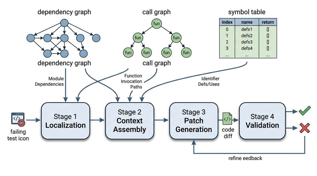
Stage 2: Context assembly. Once we have identified the relevant code locations, we assemble a context window that gives the LLM enough information to generate a correct patch. This includes the target function, its callers and callees (from the call graph), type definitions it references (from the symbol table), relevant test files, and the issue description itself. The total context must fit within the model's window, so prioritization is essential.

Stage 3: Patch generation. The LLM generates a candidate patch, typically as a unified diff (a standard text format showing added and removed lines with + and - prefixes) or as complete replacement code for the affected functions. Multiple candidates may be generated (recall pass@k (the probability that at least one of \(k\) generated samples passes all tests, as introduced in Section 8.1)) and ranked by the model's confidence or by additional heuristics.

Stage 4: Validation. Each candidate patch is applied to the repository and the test suite is run. Patches that break existing tests are rejected. Patches that pass all existing tests but do not add new tests for the fix are flagged for human review. The ideal patch passes all existing tests and includes a new test that fails before the fix and passes after. As shown in Figure 8.2, failure diagnostics from validation feed back into Stage 3 for iterative refinement.

from dataclasses import dataclass


@dataclass
class Issue:
    """A simplified representation of a GitHub issue."""
    title: str
    body: str
    labels: list[str]


@dataclass
class PatchCandidate:
    """A candidate patch generated by a code model."""
    file_path: str
    original_code: str
    patched_code: str
    explanation: str
    confidence: float


def localize_issue(issue: Issue,
                   repo_graph: RepoGraph,
                   top_k: int = 10) -> list[str]:
    """Identify files most relevant to an issue using keyword + graph search.

    A production system would use embedding similarity;
    this simplified version uses keyword matching augmented
    with graph-based expansion.
    """
    keywords = set(issue.title.lower().split()
                   + issue.body.lower().split())
    # Remove common stop words
    keywords -= {"the", "a", "an", "is", "in", "to", "and", "of",
                 "for", "on", "with", "this", "that", "it"}

    # Score each symbol by keyword overlap
    scores: dict[str, float] = {}
    for key, sym in repo_graph.symbols.items():
        name_tokens = set(sym.name.lower().split("_"))
        overlap = len(keywords & name_tokens)
        if overlap > 0:
            scores[sym.file] = scores.get(sym.file, 0) + overlap

    # Expand via dependency graph: if file F is relevant,
    # boost files that import F or that F imports
    expanded_scores = dict(scores)
    for f, score in scores.items():
        for neighbor in repo_graph.impact_set(f):
            expanded_scores[neighbor] = (
                expanded_scores.get(neighbor, 0) + score * 0.3
            )

    # Return top-k files sorted by score
    ranked = sorted(expanded_scores.items(),
                    key=lambda x: x[1], reverse=True)
    return [f for f, _ in ranked[:top_k]]


def validate_patch(patch: PatchCandidate,
                   test_runner: callable) -> dict:
    """Validate a patch by running the test suite.

    Returns a dict with pass/fail status and test results.
    """
    # Apply the patch (in a real system, use a temp worktree)
    results = {
        "tests_passed": False,
        "new_failures": [],
        "has_new_test": False,
    }

    try:
        test_output = test_runner(patch.file_path, patch.patched_code)
        results["tests_passed"] = test_output["all_passed"]
        results["new_failures"] = test_output.get("failures", [])
        results["has_new_test"] = test_output.get("new_tests", 0) > 0
    except Exception as e:
        results["error"] = str(e)

    return results

4. Test-Guided Program Repair

Test-guided program repair takes the validation step further: instead of using tests only to filter generated patches, it uses failing tests as the specification for the repair itself. Given a failing test, the repair system identifies which code the test exercises (via the call graph), generates candidate patches for that code, and iterates until a patch makes the test pass without breaking other tests.

The formal setup: let \(T_{\text{pass}}\) be the set of currently passing tests and \(T_{\text{fail}}\) be the set of failing tests (indicating the bug). A correct repair is a patch \(p\) such that:

The challenge is that many patches satisfy \(T_{\text{fail}}\) (they make the failing test pass) but violate some \(t \in T_{\text{pass}}\) (they break existing functionality). These are plausible but incorrect patches. A strong test suite reduces this risk but cannot eliminate it entirely, because tests are themselves incomplete specifications. The best repair systems address this by generating patches that include new tests. If the repair is correct, those tests encode the invariant that the bug violated.

import subprocess
import tempfile
import shutil
from pathlib import Path


def test_guided_repair(repo_path: str,
                       failing_test: str,
                       generate_patch: callable,
                       max_attempts: int = 5) -> PatchCandidate | None:
    """Iteratively generate and test patches until one passes.

    Args:
        repo_path: Path to the repository root
        failing_test: The test identifier (e.g., "tests/test_auth.py::test_login")
        generate_patch: A callable that takes (repo_path, test_id, feedback)
            and returns a PatchCandidate
        max_attempts: Maximum number of repair attempts

    Returns:
        A validated PatchCandidate, or None if all attempts fail
    """
    feedback = f"Failing test: {failing_test}"

    for attempt in range(max_attempts):
        # Generate a candidate patch
        patch = generate_patch(repo_path, failing_test, feedback)
        if patch is None:
            continue

        # Apply patch in an isolated copy
        with tempfile.TemporaryDirectory() as tmp:
            work_dir = Path(tmp) / "repo"
            shutil.copytree(repo_path, work_dir)

            # Write the patched file
            patched_file = work_dir / patch.file_path
            patched_file.write_text(patch.patched_code, encoding="utf-8")

            # Run the full test suite
            result = subprocess.run(
                ["python", "-m", "pytest", "--tb=short", "-q"],
                cwd=work_dir,
                capture_output=True,
                text=True,
                timeout=120,
            )

            if result.returncode == 0:
                print(f"Repair succeeded on attempt {attempt + 1}")
                return patch

            # Extract failure info to guide the next attempt
            feedback = (
                f"Attempt {attempt + 1} failed.\n"
                f"Test output:\n{result.stdout[-1000:]}\n"
                f"Errors:\n{result.stderr[-500:]}"
            )
            print(f"Attempt {attempt + 1}: {result.stdout.splitlines()[-1]}")

    return None  # All attempts exhausted

Notice the feedback loop: each failed attempt produces diagnostic information (test output, error messages) that is fed back to the patch generator. This is the generate-test-refine cycle that characterizes modern coding agents. The agent does not need to get the patch right on the first try; it learns from each failure. This iterative approach connects directly to the exploration-exploitation framework from Section 1.2, where exploration means sampling diverse candidate solutions and exploitation means focusing on the most promising ones: each repair attempt explores a different region of patch space, and the feedback signal guides exploitation toward regions where previous attempts came closest to passing.

5. Building a Repository Map

The techniques above assume the agent already knows which files to examine. On an unfamiliar codebase, it first needs a structural overview. A repository map provides that overview: a compact summary combining elements from all three graph structures into a format readable by both developers and LLMs, sized to fit within a single context window.

def generate_repo_map(repo_graph: RepoGraph,
                      max_depth: int = 2) -> str:
    """Generate a concise repository map showing file structure and key symbols.

    The map shows each file with its classes and top-level functions,
    annotated with dependency and call information.
    """
    lines = ["# Repository Map\n"]

    # Group symbols by file
    file_symbols: dict[str, list[SymbolInfo]] = {}
    for key, sym in repo_graph.symbols.items():
        file_symbols.setdefault(sym.file, []).append(sym)

    # Sort files for consistent output
    for file_path in sorted(file_symbols.keys()):
        symbols = file_symbols[file_path]
        lines.append(f"## {file_path}")

        # Show imports (dependencies)
        deps = [imp for src, imp in repo_graph.dep_edges
                if src == file_path]
        if deps:
            lines.append(f"  imports: {', '.join(deps[:5])}")

        # Show classes and functions
        classes = [s for s in symbols if s.kind == "class"]
        functions = [s for s in symbols if s.kind == "function"]

        for cls in classes:
            lines.append(f"  class {cls.name} (line {cls.line})")
            # Find methods belonging to this class
            methods = [s for s in functions
                       if s.line > cls.line
                       and s.name != cls.name]
            for m in methods[:max_depth * 3]:
                # Count outgoing calls
                call_key = f"{file_path}::{m.name}"
                callees = [c for caller, c in repo_graph.call_edges
                           if caller == call_key]
                call_info = (f" -> {', '.join(callees[:3])}"
                             if callees else "")
                lines.append(f"    def {m.name} (line {m.line})"
                             f"{call_info}")

        # Top-level functions (not inside classes)
        for func in functions:
            if not any(func.line > c.line for c in classes):
                lines.append(f"  def {func.name} (line {func.line})")

        lines.append("")

    return "\n".join(lines)

A well-constructed repository map serves as the AI agent's mental model of the codebase. It answers the question "where should I look?" before the agent reads any file in full. This two-stage approach (map first, then read relevant files) mirrors how experienced developers navigate unfamiliar codebases: scan the directory structure, read the README, then dive into specific files. We formalize this retrieval strategy as part of the Discovery Workbench's code analysis pipeline in Chapter 16.

Exercises

1. (Conceptual) Explain why a static call graph over-approximates while a dynamic call graph under-approximates. Give a concrete Python example where the two graphs differ, using polymorphism or dynamic dispatch.
2. (Coding) Extend the RepoGraph class from Listing 8.5 to compute a change impact score for each file: the number of files in its transitive reverse-dependency closure. Run it on a small open-source Python project (e.g., httpx or fastapi) and identify the five files with the highest impact scores. Explain why high-impact files deserve more careful AI-generated patches.
3. (Analysis) The issue-to-patch pipeline in Listing 8.7 uses keyword matching for localization. Propose an embedding-based alternative that encodes function signatures and issue text into a shared vector space. What embedding model would you use? How would you handle the vocabulary mismatch between natural-language issue descriptions and code identifiers?