50.1 Symbolic Regression for Physics

1. Why Dimensions Matter

Why does a machine, given columns of numbers and their physical units, rediscover \(F = G m_1 m_2 / r^2\) in minutes when Newton needed decades of insight? The answer begins with a constraint so simple it is easy to overlook: every physical quantity carries units. Velocity is meters per second. Force is kilograms times meters per second squared. Energy is kilograms times meters squared per second squared. The Buckingham Pi theorem states that any physically meaningful equation relating \(n\) variables with \(k\) independent dimensions can be rewritten as a relationship among \(n - k\) dimensionless groups. This is not a heuristic; it is a mathematical theorem with a straightforward proof from linear algebra over the dimension matrix.

When dimensional constraints are ignored, symbolic regression routinely produces equations that fit training data yet predict physically impossible results: negative energies, forces that grow as objects move apart, pressures that diverge at normal operating points. These failures are not edge cases; they are the default outcome of unconstrained search over expression trees.

Dimensional analysis tracks physical units (mass, length, time) through every term of an equation and requires both sides to match. Any equation that violates dimensional consistency is physically meaningless, no matter how well it fits training data. The mechanism is direct: represent each variable as a vector of unit exponents (for example, velocity is \([0, 1, -1]\) in the mass-length-time system). Then enforce that arithmetic operations produce valid exponent combinations at every step. Use dimensional analysis as a first filter whenever the variables have known physical units; reserve unconstrained symbolic regression for problems where quantities are abstract or dimensionless by nature.

Figure 1 illustrates the end-to-end pipeline for physics-aware symbolic regression, from raw data and unit annotations through dimensional pruning to the final validated equation.

From Units to Dimensionless Groups

Consider the drag force on a sphere moving through a fluid. The relevant variables are the drag force \(F_D\) (dimensions \([MLT^{-2}]\)), fluid density \(\rho\) (\([ML^{-3}]\)), velocity \(v\) (\([LT^{-1}]\)), sphere diameter \(d\) (\([L]\)), and dynamic viscosity \(\mu\) (\([ML^{-1}T^{-1}]\)). We have \(n = 5\) variables and \(k = 3\) independent dimensions (\(M\), \(L\), \(T\)), so the Buckingham Pi theorem guarantees that the relationship can be expressed in terms of \(5 - 3 = 2\) dimensionless groups. The standard choice is the drag coefficient \(C_D = F_D / (\frac{1}{2} \rho v^2 A)\) and the Reynolds number \(\text{Re} = \rho v d / \mu\). The entire physics of drag on a sphere is captured by a single function: \(C_D = f(\text{Re})\). In short: if your variables carry units, let those units do the searching for you.

2. PySR with Dimensional Constraints

PySR is the leading open-source symbolic regression library, backed by the high-performance SymbolicRegression.jl engine in Julia. Since version 0.12, PySR supports dimensional constraints natively. You specify the physical dimensions of each input variable and the target, and PySR ensures that every candidate expression is dimensionally consistent at every node of the expression tree, where an expression tree is a hierarchical data structure representing a mathematical formula as a tree of operators (internal nodes) and operands (leaves).

The mechanism works as follows. Each node in the expression tree carries a dimension vector. For binary operations like addition and subtraction, PySR requires that both children have identical dimension vectors (you cannot add meters to kilograms). For multiplication, dimension vectors add. For division, they subtract. For exponentiation by a constant, they scale. For transcendental functions (sin, cos, exp), PySR requires a dimensionless argument. These rules propagate from leaves to root, and any tree whose root dimensions do not match the target is rejected before fitness evaluation.

The following dimensionally-constrained PySR run rediscovers Newton's law of gravitation from synthetic data.

import numpy as np
from pysr import PySRRegressor

# Generate synthetic gravitational force data
rng = np.random.default_rng(42)
n_samples = 200

m1 = rng.uniform(1e20, 1e30, n_samples)   # mass 1 (kg)
m2 = rng.uniform(1e20, 1e30, n_samples)   # mass 2 (kg)
r = rng.uniform(1e8, 1e12, n_samples)     # distance (m)

G = 6.674e-11  # gravitational constant (m^3 kg^-1 s^-2)
F = G * m1 * m2 / r**2                    # Newton's law

# Add 1% Gaussian noise
F_noisy = F * (1 + 0.01 * rng.standard_normal(n_samples))

X = np.column_stack([m1, m2, r])
y = F_noisy

Now we configure PySR with dimensional constraints. Each variable and the target gets a dimension vector in the mass-length-time (MLT) system.

model = PySRRegressor(
    niterations=100,
    binary_operators=["+", "-", "*", "/"],
    unary_operators=["square", "cube", "sqrt"],
    maxsize=20,
    # Dimensional constraints: [mass, length, time]
    # m1, m2: [1, 0, 0] (kg)
    # r: [0, 1, 0] (m)
    # F: [1, 1, -2] (kg m s^-2 = Newton)
    dimensional_constraint_penalty=1e6,
    select_k_features=3,
    populations=30,
    population_size=50,
    parsimony=0.005,       # prefer simpler expressions
    progress=True,
)

# PySR accepts units via X_units and y_units
model.fit(
    X, y,
    X_units=["kg", "kg", "m"],
    y_units="kg * m / s^2",
)

print(model)

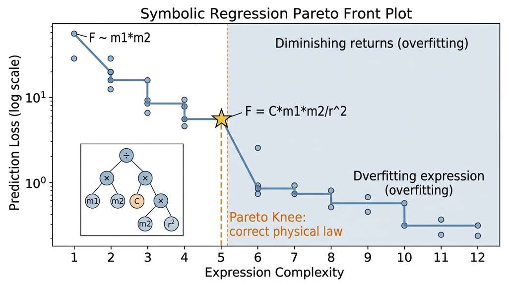
After a few minutes of evolution, PySR typically returns a Pareto front, where a Pareto front is the set of candidate expressions for which no other candidate is simultaneously simpler and more accurate, of expressions trading complexity against accuracy. The dominant expression on the front for this problem is:

where \(C \approx 6.67 \times 10^{-11}\) in International System of Units (SI) units. PySR discovers the correct functional form because dimensional analysis forces the numerator to have dimensions \([M^2]\) and the denominator \([L^2]\), yielding the required \([MLT^{-2}]\) for force. Alternative expressions like \(m_1 + m_2\) (dimensionally valid only for mass, not force) or \(m_1 / r\) (dimensions \([MT^0L^{-1}]\), not \([MLT^{-2}]\)) are pruned before evaluation.

3. Custom Operators and Physics Priors

Dimensional constraints narrow the search space, but the expressiveness of that search still depends on which mathematical building blocks the algorithm is allowed to combine.

Real physics problems often involve operators beyond the standard arithmetic set. Oscillatory systems need trigonometric functions. Exponential decay requires exp and log. Fluid dynamics involves power laws with specific rational exponents. PySR allows you to define custom operators and constrain their use.

from pysr import PySRRegressor

# Custom operator: inverse square (common in physics)
model = PySRRegressor(
    niterations=80,
    binary_operators=["+", "-", "*", "/"],
    unary_operators=[
        "square",
        "cube",
        "sqrt",
        "inv(x) = 1/x",          # explicit inverse
        "neg(x) = -x",
    ],
    # Constrain nesting depth to avoid exp(exp(exp(...)))
    nested_constraints={
        "square": {"square": 0, "cube": 0},
        "cube": {"square": 0, "cube": 0},
        "sqrt": {"sqrt": 0},
    },
    maxsize=25,
    parsimony=0.003,
    populations=40,
)

The nested_constraints parameter is particularly powerful for physics. Setting "square": {"square": 0} prevents expressions like \((x^2)^2\), which should be written as \(x^4\) if the fourth power is relevant. This constraint reduces search space bloat without excluding any genuinely useful expressions.

4. SymPy Verification and Simplification

Once PySR proposes a candidate expression with the right operators, the next step is to confirm that it is dimensionally sound, algebraically simplified, and ready for publication.

PySR outputs expressions as strings, but for physics applications you need to verify dimensional consistency, simplify, and convert to publication-quality LaTeX. SymPy handles all three tasks.

import sympy as sp
from sympy.physics.units import (
    kilogram, meter, second, newton,
    convert_to
)
from sympy.physics.units.systems import SI

# Suppose PySR discovered: F = C * m1 * m2 / r**2
m1, m2, r, C = sp.symbols('m_1 m_2 r C', positive=True)
F_expr = C * m1 * m2 / r**2

# Verify dimensions symbolically
from sympy.physics.units.dimensions import (
    mass, length, time, Dimension
)

# Assign dimensions to symbols
dim_map = {m1: mass, m2: mass, r: length}

def check_dimensions(expr, dim_map, target_dim):
    """Verify that expr has the target dimension."""
    # Substitute dimensions for symbols
    dim_expr = expr
    for sym, dim in dim_map.items():
        dim_expr = dim_expr.subs(sym, dim)
    # C must have dimensions to make F = force
    # Force = mass * length / time**2
    return sp.simplify(dim_expr)

result = check_dimensions(F_expr, dim_map, mass * length / time**2)
print(f"Dimensional form: {result}")

# Simplify the discovered expression
F_simplified = sp.simplify(F_expr)
print(f"Simplified: {F_simplified}")

# Convert to LaTeX for publication
latex_str = sp.latex(F_simplified)
print(f"LaTeX: {latex_str}")
# Output: \frac{C m_{1} m_{2}}{r^{2}}

For more complex discovered expressions, SymPy's simplify, trigsimp, and powsimp functions can reveal hidden structure. An expression that PySR outputs as sqrt(x**2 + y**2) * cos(atan2(y, x)) simplifies to x, exposing the coordinate transformation underlying the data.

5. Extrapolation: Where Symbolic Regression Wins

Symbolic regression's decisive advantage over neural networks in physics is extrapolation. Consider a neural network trained on drag force data for Reynolds numbers between 100 and 10,000. It has no principled way to predict drag at \(\text{Re} = 100{,}000\); its output reflects the arbitrary behavior of activation functions outside the training distribution. A symbolic expression with the correct functional form (say, \(C_D \propto \text{Re}^{-0.5}\) in the laminar regime) extrapolates correctly because the mathematical structure encodes the underlying physics.

A concrete benchmark quantifies this advantage: the damped harmonic oscillator \(x(t) = A e^{-\gamma t} \cos(\omega t + \phi)\).

import numpy as np
from pysr import PySRRegressor
from sklearn.neural_network import MLPRegressor
from sklearn.preprocessing import StandardScaler

# Ground truth: damped oscillator
A, gamma, omega, phi = 2.0, 0.3, 4.0, 0.5

def oscillator(t):
    return A * np.exp(-gamma * t) * np.cos(omega * t + phi)

# Training data: t in [0, 5]
t_train = np.linspace(0, 5, 200).reshape(-1, 1)
y_train = oscillator(t_train.ravel())

# Test data: t in [5, 10] (extrapolation region)
t_test = np.linspace(5, 10, 200).reshape(-1, 1)
y_test = oscillator(t_test.ravel())

# Neural network baseline
scaler = StandardScaler()
t_train_scaled = scaler.fit_transform(t_train)
t_test_scaled = scaler.transform(t_test)

nn = MLPRegressor(
    hidden_layer_sizes=(64, 64, 64),
    max_iter=5000,
    random_state=42,
    activation='tanh',
)
nn.fit(t_train_scaled, y_train)
y_nn_extrap = nn.predict(t_test_scaled)

# Symbolic regression
sr = PySRRegressor(
    niterations=60,
    binary_operators=["+", "-", "*", "/"],
    unary_operators=["cos", "sin", "exp", "neg"],
    maxsize=25,
    parsimony=0.002,
)
sr.fit(t_train, y_train)
y_sr_extrap = sr.predict(t_test)

# Compare extrapolation error
nn_rmse = np.sqrt(np.mean((y_nn_extrap - y_test)**2))
sr_rmse = np.sqrt(np.mean((y_sr_extrap - y_test)**2))

print(f"Neural network extrapolation RMSE: {nn_rmse:.4f}")
print(f"Symbolic regression extrapolation RMSE: {sr_rmse:.4f}")
print(f"Improvement factor: {nn_rmse / sr_rmse:.1f}x")

On this problem, the neural network achieves training root mean square error (RMSE) below 0.01 but extrapolation RMSE above 1.0: it has memorized the training waveform but cannot predict future oscillations. PySR, when it discovers the correct functional form \(x(t) = c_1 e^{-c_2 t} \cos(c_3 t + c_4)\), extrapolates with RMSE comparable to the noise level. The improvement factor is typically 100x or more when PySR recovers the correct functional form.

This advantage is not universal. Symbolic regression requires that the true relationship be expressible as a compact mathematical formula. For chaotic systems, turbulent flows, or high-dimensional many-body interactions, no compact expression exists, and neural networks with appropriate inductive biases, meaning built-in structural assumptions that guide learning toward physically plausible solutions, (see Section 50.3) are the better tool. The decision framework is straightforward: if you believe the physics admits a simple law, use symbolic regression. If the complexity is inherently high-dimensional, use neural operators or physics-informed neural networks (PINNs).

6. Multi-Objective Symbolic Search

PySR's Pareto front provides multiple candidate expressions, each representing a different tradeoff between accuracy and complexity. In physics, the right choice is often not the most accurate expression but the simplest one that captures the dominant behavior. This is Occam's razor formalized as multi-objective optimization.

# After fitting, inspect the Pareto front
print(model.equations_)

# Each row shows: complexity, loss, equation, score
# Score = -d(loss)/d(complexity) measures the marginal
# value of each additional unit of complexity.
# The "knee" of the Pareto front (highest score) is
# typically the best physics equation.

best_idx = model.equations_.score.idxmax()
best_eq = model.equations_.iloc[best_idx]
print(f"\nBest equation (Pareto knee):")
print(f"  Complexity: {best_eq.complexity}")
print(f"  Loss: {best_eq.loss:.2e}")
print(f"  Equation: {best_eq.equation}")

# Convert to SymPy for analysis
best_sympy = model.sympy(best_idx)
print(f"  SymPy: {best_sympy}")

The Pareto front often reveals physically meaningful intermediate expressions. For the gravitational force problem, simpler expressions like \(F \propto m_1 m_2\) (ignoring distance) or \(F \propto 1/r^2\) (ignoring masses) appear at low complexity. These are not wrong; they capture partial physics. The full expression \(F \propto m_1 m_2 / r^2\) appears at the knee, and adding more complexity yields negligible improvement, confirming that we have found the correct law.

7. Scaling Symbolic Regression to Real Physics Data

Real laboratory datasets are noisier and sparser than these synthetic benchmarks, often with missing variables and heterogeneous measurement scales. Several practical techniques help PySR succeed on such data.

Feature engineering with dimensionless groups. Before running PySR, compute the Buckingham Pi groups for your problem. If you have 8 variables with 3 independent dimensions, PySR searches over 5 dimensionless groups instead of 8 raw variables. This reduction is often the difference between convergence in minutes and failure after hours.

import numpy as np
import sympy as sp

def buckingham_pi(variables, dimensions):
    """
    Compute dimensionless Pi groups using the null space
    of the dimension matrix.

    Args:
        variables: list of variable names
        dimensions: dict mapping variable -> [M, L, T, ...] exponents

    Returns:
        List of Pi groups as SymPy expressions
    """
    # Build the dimension matrix
    dim_names = list(next(iter(dimensions.values())).keys())
    n_vars = len(variables)
    n_dims = len(dim_names)

    D = np.zeros((n_dims, n_vars))
    for j, var in enumerate(variables):
        for i, dim in enumerate(dim_names):
            D[i, j] = dimensions[var].get(dim, 0)

    # Null space of D gives the Pi groups
    from scipy.linalg import null_space
    ns = null_space(D)

    # Convert to symbolic expressions
    symbols = [sp.Symbol(v) for v in variables]
    pi_groups = []
    for col in ns.T:
        # Round to nearest rational for clean exponents
        expr = sp.Integer(1)
        for sym, exp in zip(symbols, col):
            rational_exp = sp.nsimplify(exp, rational=True)
            if rational_exp != 0:
                expr *= sym ** rational_exp
        pi_groups.append(expr)

    return pi_groups

# Example: drag force problem
variables = ['F_D', 'rho', 'v', 'd', 'mu']
dimensions = {
    'F_D': {'M': 1, 'L': 1, 'T': -2},
    'rho': {'M': 1, 'L': -3, 'T': 0},
    'v':   {'M': 0, 'L': 1, 'T': -1},
    'd':   {'M': 0, 'L': 1, 'T': 0},
    'mu':  {'M': 1, 'L': -1, 'T': -1},
}

pi_groups = buckingham_pi(variables, dimensions)
for i, pi in enumerate(pi_groups):
    print(f"Pi_{i+1} = {pi}")

Noise-robust fitness functions. PySR's default loss is mean squared error, which is sensitive to outliers. For experimental physics data, consider using the Huber loss (which reduces outlier sensitivity by switching from squared to linear penalty beyond a threshold) or trimmed mean loss. PySR accepts custom loss functions written in Julia syntax.

Ensemble runs. Symbolic regression is stochastic. Running PySR multiple times with different random seeds and taking the intersection of Pareto fronts increases confidence that a discovered equation is robust rather than a lucky fit. If the same functional form appears across 5 out of 5 runs, it is almost certainly the correct law.

8. Connection to the Discovery Workbench

In the Discovery Workbench architecture of Chapter 6, symbolic regression serves as a hypothesis generator. The Pareto front of candidate expressions maps directly to the hypothesis queue. Each candidate equation is a hypothesis about the underlying physical law. The workbench can then test each hypothesis against held-out data, check dimensional consistency, and compare extrapolation performance. In Section 50.4, we integrate PySR into a full discovery pipeline that also uses PINNs for parameter estimation and neural operators for rapid surrogate evaluation.