A physics-informed neural network (PINN) (Section 50.2) learns the solution to one partial differential equation (PDE) instance: one set of initial conditions, one set of boundary conditions, one geometry. Change any of these and you must retrain. A neural operator learns the mapping from input functions (initial conditions, forcing terms, coefficient fields) to output functions (the PDE solution). Once trained, it generalizes to new inputs without retraining. This is the difference between learning a function \(u = f(x)\) and learning a functional \(\mathcal{G}: \mathcal{A} \to \mathcal{U}\) that maps between infinite-dimensional function spaces. The theoretical foundation is the universal approximation theorem for operators (Chen and Chen, 1995), which guarantees that neural networks can approximate any continuous nonlinear operator to arbitrary accuracy.
1. From Functions to Operators
What if you could hand a neural network an entire pressure field, temperature map, or velocity profile and get back the solution to a completely new configuration in milliseconds, without ever re-solving the underlying equations? That is exactly what a neural operator does: instead of learning a mapping between finite-dimensional vectors (\(f: \mathbb{R}^n \to \mathbb{R}^m\)), it learns a mapping between function spaces, \(\mathcal{G}: \mathcal{A} \to \mathcal{U}\), where \(\mathcal{A}\) and \(\mathcal{U}\) are spaces of functions defined on some domain \(D \subset \mathbb{R}^d\).
A neural operator takes an entire function as input and produces an entire function as output. Unlike conventional networks that map fixed-size vectors, it operates on function spaces. Most physics and engineering problems require solving the same equation repeatedly for different configurations. A neural operator amortizes this cost by learning the solution map itself: each new configuration requires only a single forward pass (milliseconds) instead of a full numerical solve (seconds to hours). The core mechanism parameterizes the integral kernel of the solution operator with a neural network. Input-output function pairs in the training data teach the network to reproduce the operator that the PDE defines. Use a neural operator instead of a classical solver when you need thousands of evaluations across varying inputs (optimization loops, uncertainty quantification, real-time control); use a classical solver when you need a single high-fidelity answer or when training data is unavailable.
Consider the steady-state Darcy flow equation, which models groundwater flow through porous media:
$$-\nabla \cdot (a(x) \nabla u(x)) = f(x), \quad x \in D$$Here \(a(x)\) is the permeability field (how easily fluid flows through the material at each point), \(u(x)\) is the pressure field (the solution), and \(f(x)\) is the source term. The operator we want to learn maps the permeability field to the pressure field: \(\mathcal{G}: a(\cdot) \mapsto u(\cdot)\). This is an operator because both the input \(a\) and the output \(u\) are functions of spatial position, not finite-dimensional vectors.
The key advantage is zero-shot generalization: once \(\mathcal{G}\) is learned, it maps any permeability field to its corresponding pressure solution, including fields never seen during training. A classical solver must re-solve the PDE from scratch for each new \(a(x)\). A neural operator evaluation takes milliseconds. In short: a neural operator learns the solution map once so that every future query costs a forward pass, not a fresh solve.
Because neural operators learn mappings between function spaces rather than between fixed grids, they are inherently resolution-invariant. A Fourier Neural Operator (FNO) trained on 64x64 grids can be evaluated on 256x256 grids (or even irregular point clouds) without retraining. The input and output functions are the mathematical objects; the grid is merely a discretization. This property is unique to operator learning and has no analogue in standard neural networks, which require inputs and outputs of fixed dimension.
Common Misconception
A frequent misunderstanding is that "resolution invariance" means an FNO trained at low resolution will produce equally accurate results when evaluated at much higher resolution. In reality, resolution invariance means the architecture can accept inputs at any resolution, but accuracy at resolutions far beyond the training distribution will degrade because the model has never seen the fine-scale features that higher resolution reveals. Always validate on a few high-resolution samples before trusting a model trained on coarser grids.
2. The Universal Approximation Theorem for Operators
Chen and Chen (1995) proved the universal approximation theorem for operators, the theoretical backbone of neural operator methods. Lu et al. (2021) later extended the result. The theorem guarantees that for any continuous nonlinear operator \(\mathcal{G}: \mathcal{A} \to \mathcal{U}\) and any \(\epsilon > 0\), a neural network architecture exists that approximates \(\mathcal{G}\) to within \(\epsilon\) in the appropriate norm.
More precisely, let \(\mathcal{A}\) be a compact set in a Banach space (a complete normed vector space, generalizing Euclidean space to infinite dimensions) and \(\mathcal{G}: \mathcal{A} \to C(K)\) be a continuous operator mapping into continuous functions on a compact set \(K\). Then \(\mathcal{G}\) can be approximated by a network of the form:
$$\mathcal{G}(a)(y) \approx \sum_{k=1}^{p} \underbrace{c_k \sigma\!\left(\sum_{j=1}^{m} \xi_{kj}\, a(x_j) + \zeta_k \right)}_{\text{branch net (encodes } a)} \cdot \underbrace{\tau_k(y)}_{\text{trunk net (encodes } y)}$$This is the DeepONet architecture: a branch network that processes the input function \(a\) (evaluated at sensor locations \(x_1, \dots, x_m\)) and a trunk network that processes the evaluation point \(y\). The output is the inner product of the branch and trunk outputs.
DeepONet is theoretically elegant, but for PDE problems on regular grids, the FNO achieves better accuracy with simpler training. The FNO is therefore the primary architecture below; DeepONet returns in Section 6.
3. Fourier Neural Operator Architecture
The key observation behind the FNO is that many PDE operators are naturally expressed in Fourier space. Convolution in physical space becomes pointwise multiplication in frequency space. The FNO exploits this by learning the operator kernel directly in the Fourier domain.
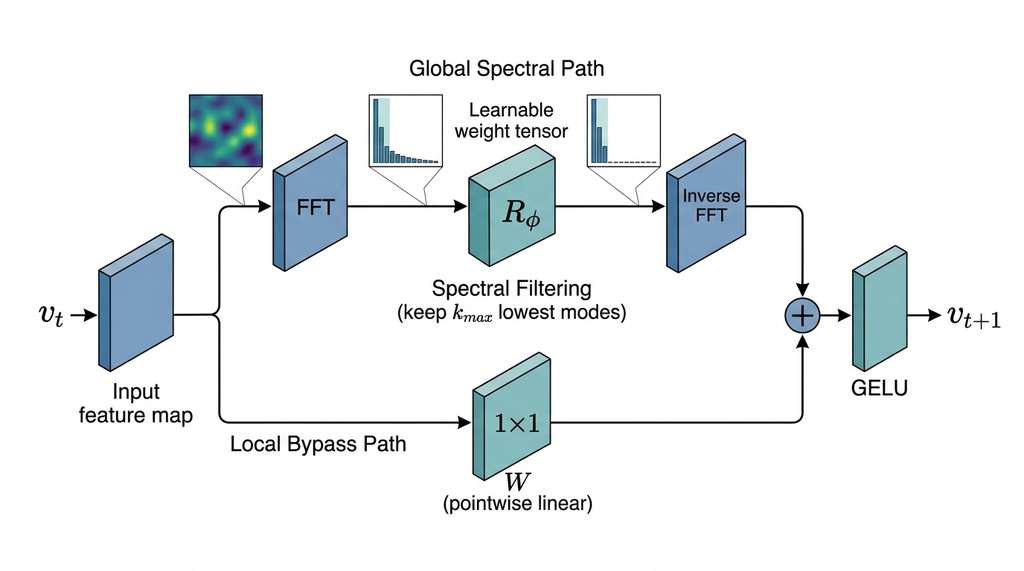
An FNO layer performs four operations, illustrated in Figure 50.3.1 below:
- Fourier transform: apply the Fast Fourier Transform (FFT) to the input function, mapping it from physical space to frequency space.
- Spectral filtering: multiply the Fourier coefficients by a learnable weight tensor \(R_\phi\), keeping only the lowest \(k_{\max}\) modes. This is the learned kernel in Fourier space.
- Inverse Fourier transform: apply the inverse FFT to return to physical space.
- Local bypass: add a pointwise linear transformation \(Wv(x)\) (a 1x1 convolution) that captures local, high-frequency interactions missed by the truncated Fourier representation.
Mental Model
Think of spectral convolution like an audio equalizer on a mixing board. An equalizer decomposes a music signal into frequency bands (bass, midrange, treble), lets you boost or cut each band independently with a slider, then recombines the adjusted bands back into a single audio signal. The FNO does the same thing with spatial data: the FFT decomposes the input field into spatial frequency components (large-scale smooth patterns are "bass," small-scale rapid variations are "treble"), the learnable weight tensor \(R_\phi\) acts as the set of sliders that boost or suppress each frequency, and the inverse FFT recombines everything into the output field. The local bypass path is like a separate "direct monitor" channel that preserves crisp transients the equalizer's limited number of bands would smear out. Training teaches the network which spatial frequencies to amplify and which to dampen for a given PDE, just as a sound engineer learns which EQ settings produce the right tonal balance for a particular recording.
Mathematically, one FNO layer maps input \(v_t\) to output \(v_{t+1}\):
$$v_{t+1}(x) = \sigma\!\Big(\underbrace{\mathcal{F}^{-1}\!\big(R_\phi \cdot \mathcal{F}(v_t)\big)(x)}_{\text{global spectral convolution}} + \underbrace{W v_t(x) + b}_{\text{local linear bypass}}\Big)$$where \(\mathcal{F}\) denotes the FFT, \(R_\phi\) is the learnable spectral weight tensor, \(W\) is a pointwise weight matrix, and \(\sigma\) is a nonlinear activation (typically Gaussian Error Linear Unit, or GELU). Stacking \(L\) such layers (typically \(L = 4\)) with a lifting layer (a pointwise linear map that projects the low-dimensional input, such as coordinates plus the coefficient field, into a higher-dimensional channel space) at the input and a projection layer (a pointwise linear map that collapses the high-dimensional channel representation back to the scalar solution field) at the output gives the complete FNO architecture.
Checkpoint
So far: an FNO layer decomposes its input into frequency components via FFT, applies a learnable spectral filter to the lowest modes, transforms back via inverse FFT, adds a local linear bypass, and passes the sum through a nonlinearity; stacking several such layers between a lifting layer and a projection layer yields the full architecture.
import torch
import torch.nn as nn
import torch.fft

class SpectralConv2d(nn.Module):
    """Spectral convolution layer for 2D FNO."""

    def __init__(self, in_channels, out_channels, modes1, modes2):
        super().__init__()
        self.in_channels = in_channels
        self.out_channels = out_channels
        self.modes1 = modes1  # number of Fourier modes (x)
        self.modes2 = modes2  # number of Fourier modes (y)

        # Learnable weights in Fourier space (complex-valued)
        scale = 1.0 / (in_channels * out_channels)
        self.weights1 = nn.Parameter(
            scale * torch.rand(in_channels, out_channels,
                               modes1, modes2, dtype=torch.cfloat)
        )
        self.weights2 = nn.Parameter(
            scale * torch.rand(in_channels, out_channels,
                               modes1, modes2, dtype=torch.cfloat)
        )

    def compl_mul2d(self, input, weights):
        """Complex multiplication in Fourier space."""
        # input: (batch, in_ch, x, y)
        # weights: (in_ch, out_ch, x, y)
        return torch.einsum("bixy,ioxy->boxy", input, weights)

    def forward(self, x):
        batch_size = x.shape[0]

        # FFT along spatial dimensions
        x_ft = torch.fft.rfft2(x)

        # Multiply relevant Fourier modes with learnable weights
        out_ft = torch.zeros(
            batch_size, self.out_channels,
            x.size(-2), x.size(-1) // 2 + 1,
            dtype=torch.cfloat, device=x.device,
        )
        # Low-frequency modes (positive frequencies)
        out_ft[:, :, :self.modes1, :self.modes2] = \
            self.compl_mul2d(
                x_ft[:, :, :self.modes1, :self.modes2],
                self.weights1,
            )
        # Low-frequency modes (negative frequencies)
        out_ft[:, :, -self.modes1:, :self.modes2] = \
            self.compl_mul2d(
                x_ft[:, :, -self.modes1:, :self.modes2],
                self.weights2,
            )

        # Inverse FFT
        x = torch.fft.irfft2(out_ft, s=(x.size(-2), x.size(-1)))
        return x


class FNO2d(nn.Module):
    """
    Fourier Neural Operator for 2D PDEs.

    Architecture:
        Lift -> [SpectralConv + Linear + Activation] x L -> Project
    """

    def __init__(self, modes1, modes2, width, n_layers=4):
        super().__init__()
        self.modes1 = modes1
        self.modes2 = modes2
        self.width = width
        self.n_layers = n_layers

        # Lifting layer: input channels -> width
        self.lift = nn.Linear(3, width)  # (x, y, a(x,y)) -> width

        # Spectral convolution layers
        self.spectral_convs = nn.ModuleList([
            SpectralConv2d(width, width, modes1, modes2)
            for _ in range(n_layers)
        ])

        # Local linear bypass (1x1 convolution)
        self.linear_layers = nn.ModuleList([
            nn.Conv2d(width, width, 1)
            for _ in range(n_layers)
        ])

        # Projection layer: width -> 1 (solution field)
        self.project = nn.Sequential(
            nn.Linear(width, 128),
            nn.GELU(),
            nn.Linear(128, 1),
        )

    def forward(self, x):
        # x shape: (batch, nx, ny, 3) = (batch, nx, ny, [x, y, a])
        batch, nx, ny, _ = x.shape

        # Lift to higher dimension
        h = self.lift(x)                    # (batch, nx, ny, width)
        h = h.permute(0, 3, 1, 2)          # (batch, width, nx, ny)

        # FNO layers
        for spectral, linear in zip(
            self.spectral_convs, self.linear_layers
        ):
            h1 = spectral(h)                # global Fourier path
            h2 = linear(h)                  # local bypass path
            h = torch.nn.functional.gelu(h1 + h2)

        # Project back to solution space
        h = h.permute(0, 2, 3, 1)          # (batch, nx, ny, width)
        h = self.project(h)                 # (batch, nx, ny, 1)

        return h.squeeze(-1)               # (batch, nx, ny)
The implementation above illustrates the mechanics, but the
neuraloperator
library provides production-ready FNO, DeepONet, and related architectures with a
clean API. A complete FNO training pipeline reduces from the 100+ lines above to
roughly 15 lines: from neuraloperator.models import FNO, configure
hyperparameters, and call trainer.train(). The library also handles
data loading for standard PDE benchmarks (Darcy flow, Navier-Stokes, Burgers),
mixed-precision training, and distributed computation.
4. Training on Darcy Flow
The Darcy flow benchmark is the standard test problem for neural operators. The input is a permeability field \(a(x, y)\) (typically a piecewise constant "checkerboard" sampled from a Gaussian random field, where the value at each spatial point is drawn from a multivariate Gaussian distribution with a prescribed spatial correlation structure), and the target is the pressure solution \(u(x, y)\) computed by a high-fidelity finite element solver. The training set contains 1,000 input-output pairs on a 64x64 grid; the test set contains 200 unseen pairs.
import torch
from torch.utils.data import DataLoader, TensorDataset

def load_darcy_flow(data_path, n_train=1000, n_test=200, resolution=64):
    """
    Load the Darcy flow benchmark dataset.

    Each sample contains:
      - a(x,y): permeability coefficient field (64x64)
      - u(x,y): pressure solution field (64x64)
    """
    data = torch.load(data_path)
    a_train = data['a'][:n_train, :resolution, :resolution]
    u_train = data['u'][:n_train, :resolution, :resolution]
    a_test = data['a'][n_train:n_train+n_test, :resolution, :resolution]
    u_test = data['u'][n_train:n_train+n_test, :resolution, :resolution]

    # Create coordinate grid
    grid_x = torch.linspace(0, 1, resolution)
    grid_y = torch.linspace(0, 1, resolution)
    grid_x, grid_y = torch.meshgrid(grid_x, grid_y, indexing='ij')

    # Stack inputs: (x, y, a(x,y))
    def make_input(a_batch):
        batch_size = a_batch.shape[0]
        gx = grid_x.unsqueeze(0).expand(batch_size, -1, -1)
        gy = grid_y.unsqueeze(0).expand(batch_size, -1, -1)
        return torch.stack([gx, gy, a_batch], dim=-1)

    x_train = make_input(a_train)
    x_test = make_input(a_test)

    return (
        DataLoader(TensorDataset(x_train, u_train),
                   batch_size=32, shuffle=True),
        DataLoader(TensorDataset(x_test, u_test),
                   batch_size=32, shuffle=False),
    )


def train_fno(model, train_loader, test_loader, n_epochs=100, lr=1e-3):
    """Train FNO with relative L2 loss (the ratio of the prediction
    error norm to the true solution norm, so 0.01 means 1% error
    regardless of solution scale)."""
    optimizer = torch.optim.Adam(model.parameters(), lr=lr,
                                  weight_decay=1e-4)
    scheduler = torch.optim.lr_scheduler.CosineAnnealingLR(
        optimizer, T_max=n_epochs
    )

    for epoch in range(n_epochs):
        model.train()
        train_loss = 0.0

        for x_batch, u_batch in train_loader:
            optimizer.zero_grad()
            u_pred = model(x_batch)

            # Relative L2 loss: ||u_pred - u_true|| / ||u_true||
            loss = torch.mean(
                torch.norm(u_pred - u_batch, dim=(-2, -1))
                / torch.norm(u_batch, dim=(-2, -1))
            )
            loss.backward()
            optimizer.step()
            train_loss += loss.item()

        scheduler.step()

        # Evaluate
        if (epoch + 1) % 10 == 0:
            model.eval()
            test_loss = 0.0
            with torch.no_grad():
                for x_batch, u_batch in test_loader:
                    u_pred = model(x_batch)
                    test_loss += torch.mean(
                        torch.norm(u_pred - u_batch, dim=(-2, -1))
                        / torch.norm(u_batch, dim=(-2, -1))
                    ).item()

            n_train_batches = len(train_loader)
            n_test_batches = len(test_loader)
            print(
                f"Epoch {epoch+1:3d} | "
                f"Train: {train_loss/n_train_batches:.4f} | "
                f"Test: {test_loss/n_test_batches:.4f}"
            )

    return model

# Instantiate and train
model = FNO2d(modes1=12, modes2=12, width=32, n_layers=4)
print(f"FNO parameters: {sum(p.numel() for p in model.parameters()):,}")
# Typically ~2.4M parameters for this configuration
On the Darcy flow benchmark, an FNO with 12 Fourier modes and 4 layers achieves a relative L2 test error (the prediction error norm divided by the true solution norm, so that 0.01 means 1% error regardless of solution scale) typically below 1.5% after 100 epochs of training. Each forward pass takes approximately 3 milliseconds on a graphics processing unit (GPU), compared to roughly 10 seconds for the finite element solver, approximately a 3000x speedup. That speed gap is the value proposition of neural operators for engineering applications: once trained, they enable real-time evaluation of PDE solutions across the design space.
5. Navier-Stokes Surrogate
Darcy flow is a steady-state, linear PDE, so the 3000x speedup above is impressive but not yet a stress test; real engineering problems demand that neural operators handle time-dependent, nonlinear dynamics as well.
The more challenging and scientifically significant benchmark is the 2D Navier-Stokes equation for incompressible viscous flow:
$$\frac{\partial w}{\partial t} + u \cdot \nabla w = \nu \Delta w + f, \quad \nabla \cdot u = 0$$where \(w = \nabla \times u\) is the vorticity (the curl of the velocity field, measuring local rotation in the fluid), \(\nu\) is the viscosity, and \(f\) is an external forcing. The operator learning task maps the vorticity at time steps \([0, T_{\text{in}}]\) to future vorticity at times \([T_{\text{in}}+1, T_{\text{out}}]\).
For this time-dependent problem, the FNO processes a stack of input time steps as channels and predicts a stack of output time steps. At viscosity \(\nu = 10^{-3}\), the flow is mildly turbulent, and the FNO typically achieves relative errors of approximately 5% for 10-step-ahead prediction. At \(\nu = 10^{-4}\) (more turbulent), errors typically rise to approximately 15%, reflecting the increasing complexity of the solution manifold.
An automotive engineer needs to evaluate the drag coefficient for 10,000 different car body shapes during an optimization campaign. Each computational fluid dynamics (CFD) simulation takes 4 hours. Running all 10,000 sequentially would require over 4 years of compute time. Instead, the engineer trains an FNO on 500 high-fidelity CFD solutions (requiring 2,000 hours, feasible on a small cluster over a weekend). The trained FNO evaluates each new shape in 50 milliseconds, completing the entire optimization campaign in under a minute. The FNO predictions have 3% relative error compared to CFD, which is acceptable for the screening phase. Only the top 20 candidate shapes are validated with full CFD, reducing total compute from 40,000 hours to 2,080 hours: a 19x speedup.
6. DeepONet: Branch-Trunk Architecture
While FNO excels on regular grids, DeepONet handles irregular sensor locations and heterogeneous input representations. The architecture consists of two sub-networks:
Branch and Trunk Sub-Networks
The branch network processes the input function \(a\), evaluated at fixed sensor locations \((x_1, \dots, x_m)\). It takes the vector \((a(x_1), \dots, a(x_m))\) and produces a feature vector \(b \in \mathbb{R}^p\).
The trunk network processes the query location \(y\) where we want to evaluate the output function. It takes \(y\) and produces a feature vector \(\tau \in \mathbb{R}^p\).
The operator output is the inner product: \(\mathcal{G}(a)(y) \approx b \cdot \tau\).
import torch
import torch.nn as nn

class DeepONet(nn.Module):
    """
    DeepONet: branch-trunk architecture for operator learning.

    Branch: processes input function at sensor locations.
    Trunk: processes query evaluation point.
    Output: dot product of branch and trunk features.
    """

    def __init__(self, n_sensors, branch_width, trunk_width, p):
        """
        Args:
            n_sensors: number of sensor locations for input function
            branch_width: hidden layer width for branch network
            trunk_width: hidden layer width for trunk network
            p: dimension of the feature vectors (branch/trunk output)
        """
        super().__init__()

        # Branch network: sensor values -> feature vector
        self.branch = nn.Sequential(
            nn.Linear(n_sensors, branch_width),
            nn.Tanh(),
            nn.Linear(branch_width, branch_width),
            nn.Tanh(),
            nn.Linear(branch_width, p),
        )

        # Trunk network: query point -> feature vector
        self.trunk = nn.Sequential(
            nn.Linear(2, trunk_width),    # 2D spatial input
            nn.Tanh(),
            nn.Linear(trunk_width, trunk_width),
            nn.Tanh(),
            nn.Linear(trunk_width, p),
        )

        # Learnable bias
        self.bias = nn.Parameter(torch.zeros(1))

    def forward(self, a_sensors, y_query):
        """
        Args:
            a_sensors: (batch, n_sensors) input function values
            y_query: (batch, n_query, 2) query locations

        Returns:
            u_pred: (batch, n_query) predicted output function values
        """
        # Branch: (batch, p)
        b = self.branch(a_sensors)

        # Trunk: (batch, n_query, p)
        tau = self.trunk(y_query)

        # Dot product: (batch, n_query)
        u_pred = torch.einsum("bp,bqp->bq", b, tau) + self.bias

        return u_pred
7. Comparing Neural Operators, PINNs, and Classical Solvers
With both FNO (optimized for regular grids) and DeepONet (flexible on irregular geometries) now in hand, the natural question is when to reach for each, and when a classical solver or a PINN remains the better tool.
The table below compares classical solvers, PINNs, FNO, and DeepONet on the Darcy flow and Navier-Stokes benchmarks.
| Property | Classical Solver (Finite Element Method, FEM) | PINN | FNO | DeepONet |
|---|---|---|---|---|
| Learns from data? | No (uses equations) | Partially | Yes | Yes |
| Requires PDE? | Yes | Yes | No (data-driven) | No (data-driven) |
| Generalizes across inputs? | Re-solve each time | Re-train | Yes (zero-shot) | Yes (zero-shot) |
| Resolution invariant? | Mesh-dependent | Mesh-free | Yes | Yes (sensor-dep.) |
| Training cost | N/A | Minutes per instance | Hours (amortized) | Hours (amortized) |
| Inference cost | Seconds to hours | Milliseconds | Milliseconds | Milliseconds |
| Accuracy (Darcy) | Reference | ~1% relative | ~1.5% relative | ~3% relative |
| Best for | Single high-fidelity run | Inverse problems | Parametric studies | Irregular domains |
The decision between classical solvers and neural operators is an amortization calculation (spreading a large upfront cost over many cheap subsequent uses, so that the per-use cost falls as the number of uses grows). Training an FNO requires generating a dataset of solved PDE instances (say, 1,000 finite element solutions at 10 seconds each = 2.8 hours), plus training time (say, 2 hours on a single GPU). This upfront cost of approximately 5 hours is paid once. After training, each new evaluation costs 3 milliseconds. The break-even point is roughly 1,800 evaluations (5 hours / 10 seconds per classical solve). For engineering optimization campaigns requiring 10,000+ evaluations, the FNO approach is 1,000x cheaper. For a one-off analysis requiring 3 evaluations, the classical solver wins.
8. Physics-Informed Neural Operators
Physics-Informed Neural Operators (PINO, Li et al., 2021) combine the physics-informed losses of PINNs with the operator learning of FNO. PINO adds PDE residual losses to the FNO training objective, enabling training with fewer data pairs and better generalization to out-of-distribution inputs.
def pino_loss(model, x_batch, u_batch, x_colloc, pde_weight=1.0):
    """
    Combined data + physics loss for PINO.

    The data loss fits available solved PDE instances.
    The physics loss enforces the PDE at collocation points
    without requiring solved reference data.
    """
    # Data loss: fit known solutions
    u_pred = model(x_batch)
    loss_data = relative_l2_loss(u_pred, u_batch)

    # Physics loss: PDE residual at unsupervised collocation points,
    # where collocation points are spatial locations sampled across
    # the domain at which the PDE residual is evaluated without
    # requiring reference solution data
    x_colloc.requires_grad_(True)
    u_colloc = model(x_colloc)

    # Compute PDE residual (Darcy flow: -div(a * grad(u)) = f)
    # a is embedded in x_colloc[:, :, :, 2]
    a_field = x_colloc[:, :, :, 2]

    # Spatial gradients via autograd
    du_dx = torch.autograd.grad(
        u_colloc.sum(), x_colloc, create_graph=True
    )[0]
    du_dx_spatial = du_dx[:, :, :, :2]  # gradients w.r.t. (x, y)

    # Divergence of (a * grad u)
    flux = a_field.unsqueeze(-1) * du_dx_spatial
    div_flux = torch.autograd.grad(
        flux.sum(), x_colloc, create_graph=True
    )[0][:, :, :, :2].sum(dim=-1)

    # PDE residual: should equal source term f
    residual = -div_flux  # simplified; f handled separately
    loss_physics = torch.mean(residual**2)

    return loss_data + pde_weight * loss_physics
PINO is particularly valuable when generating training data is expensive. Instead of solving 1,000 PDE instances, you can solve 100 and supplement with physics-informed collocation at 10,000 unsupervised points. The physics loss acts as a regularizer that guides the operator toward physically consistent solutions in data-sparse regions of the input space.
Research Frontier
Transformer-based neural operators are rapidly closing the gap with FNO on complex, multi-scale PDEs. The Transolver (Wu et al., "Transolver: A Fast Transformer Solver for PDEs on General Geometries," ICML 2024) replaces spectral convolution with a physics-aware attention mechanism that adaptively partitions the spatial domain into learned slices, each attending to regions of similar physical behavior. This allows Transolver to handle irregular meshes, complex 3D geometries (car bodies, airfoils, fluid-structure interactions), and multi-scale phenomena that challenge the FNO's reliance on uniform grids and global Fourier modes. On standard benchmarks, Transolver matches or exceeds FNO accuracy while generalizing to unstructured meshes without architectural changes, pointing toward a unified neural operator that works across grid types, geometries, and PDE families.
9. Connecting to Engineering Design
These architectural advances are compelling on their own, but the real payoff comes when neural operators slot into a larger engineering workflow where speed per evaluation directly determines how many design candidates can be explored.
Neural operators transform engineering design by enabling real-time PDE evaluation within optimization loops. The workflow is:
- Generate training data: run the classical solver for a representative sample of design configurations.
- Train the operator: fit an FNO or DeepONet to map design parameters to performance metrics.
- Optimize: run gradient-based or Bayesian optimization over the trained surrogate, evaluating thousands of candidates in seconds.
- Validate: run the classical solver on the top candidates to verify the surrogate's predictions.
This four-step loop is the foundation of the physics discovery pipeline in Section 50.4, where we combine PySR for law discovery, PINNs for parameter estimation, FNO for surrogate modeling, and BoTorch for optimization into a single integrated pipeline.
Try It: Train an FNO on the 1D Burgers Equation
Build a minimal neural operator from scratch in under an hour using only PyTorch and NumPy.
- Generate training data. Write a simple finite-difference solver for the 1D viscous Burgers equation \(u_t + u\,u_x = \nu\,u_{xx}\) on \([0, 1]\) with periodic boundary conditions, viscosity \(\nu = 0.01\), and 256 grid points. Generate 1,200 samples by drawing random initial conditions from a truncated Fourier series with 5 random modes. Save the initial condition and the solution at \(t = 1.0\) for each sample.
- Implement a 1D spectral convolution layer. Adapt the
SpectralConv2dclass from this section to 1D: usetorch.fft.rfftandtorch.fft.irfftinstead ofrfft2/irfft2, and keep only one set of learnable weights for 16 Fourier modes. - Build and train. Stack 4 spectral convolution layers with GELU activations, a lifting layer (
nn.Linear(2, 64)mapping spatial coordinate plus initial condition to width 64), and a projection layer back to 1 channel. Train for 200 epochs with the Adam optimizer (lr=1e-3) and relative L2 loss on 1,000 training pairs. - Evaluate. Test on the 200 held-out samples. Compute the mean relative L2 error (target: below 3%). Plot three examples showing the true solution, the FNO prediction, and the pointwise error.
- Test resolution transfer. Evaluate your trained model (trained on 256-point grids) on 512-point and 1024-point grids by interpolating the initial condition onto the finer grid, running the forward pass, and comparing against the finite-difference solution at the finer resolution. Observe how accuracy changes with resolution.
Exercise 50.3.1
An FNO is trained on 1,000 Darcy flow samples at 64x64 resolution with 12 Fourier modes
per spatial dimension. The spectral weight tensor \(R_\phi\) in each layer has shape
(in_channels, out_channels, modes1, modes2) with complex-valued entries.
If the network width is 32 (meaning in_channels = out_channels = 32), how
many learnable real-valued parameters does a single SpectralConv2d layer
contain? (Count both weights1 and weights2.)
Hint
Each complex number has two real components (real and imaginary parts). Each weight
tensor has shape (32, 32, 12, 12). There are two such tensors per layer
(weights1 for positive frequencies and weights2 for negative
frequencies). Multiply the total number of complex parameters by 2 to get real-valued
parameter count.
Step-Through: One FNO Layer on a 4-Point 1D Signal
Trace through a single 1D FNO layer with a tiny input to see each operation concretely. Suppose our input signal is \(v = [1.0,\; 0.0,\; -1.0,\; 0.0]\) on a 4-point grid, with 1 input channel, 1 output channel, and \(k_{\max} = 2\) retained Fourier modes.
Step 1 (FFT): Compute the real FFT of \(v\). The result is \(\hat{v} = [0.0,\; (1.0 - 1.0i),\; 0.0]\) (three complex coefficients for a length-4 real signal: DC, mode 1, and Nyquist).
Step 2 (Spectral filtering): With \(k_{\max} = 2\), we keep modes 0 and 1. Suppose the learnable weight \(R_\phi = [0.5,\; (0.0 + 1.0i)]\) for these two modes. Multiply pointwise: filtered coefficients become \([0.0 \times 0.5,\; (1.0 - 1.0i)(0.0 + 1.0i)] = [0.0,\; (1.0 + 1.0i)]\). The Nyquist mode is zeroed: \([0.0,\; (1.0 + 1.0i),\; 0.0]\).
Step 3 (Inverse FFT): Apply the inverse real FFT to get \(v_{\text{spectral}} = [0.5,\; 0.5,\; -0.5,\; -0.5]\).
Step 4 (Local bypass): Apply a pointwise linear weight \(W = 0.3\): \(v_{\text{local}} = [0.3,\; 0.0,\; -0.3,\; 0.0]\).
Step 5 (Combine + activate): Sum the two paths and apply GELU: \(v_{\text{out}} = \text{GELU}([0.8,\; 0.5,\; -0.8,\; -0.5]) \approx [0.72,\; 0.35,\; -0.18,\; -0.15]\). The spectral path captured the global shape; the bypass preserved local detail.
Real-World Application: Weather Forecasting with FourCastNet
NVIDIA's FourCastNet system uses an Adaptive Fourier Neural Operator (AFNO), a variant of the FNO that replaces fixed spectral filters with channel-mixing attention in the frequency domain, to produce global weather forecasts at 0.25-degree resolution (roughly 25 km). Trained on 40 years of ERA5 reanalysis data (a global atmospheric dataset produced by the European Centre for Medium-Range Weather Forecasts that combines historical observations with numerical model output), FourCastNet generates a 7-day forecast in under 2 seconds on a single GPU, compared to hours of supercomputer time for traditional numerical weather prediction models. The system has demonstrated competitive accuracy with the Integrated Forecasting System (IFS) for variables such as surface wind speed and precipitation, making neural operators a viable path toward real-time ensemble weather prediction at scale. (As of 2024, Google DeepMind's GraphCast and GenCast have surpassed FourCastNet on many forecast metrics, achieving accuracy competitive with the best operational numerical weather models while retaining the millisecond-scale inference advantage of neural operators.)
The Operator That Outsmarted Its Training Data
When Li et al. first tested FNO on turbulent Navier-Stokes flows (\(\nu = 10^{-5}\)), they noticed something unexpected: the FNO's predictions were occasionally smoother than the reference solutions, yet produced lower error on downstream quantities like energy spectra. The likely explanation was that the reference solver's grid was too coarse for that viscosity, introducing numerical artifacts that the FNO, having learned the underlying operator from many samples, effectively filtered out. In this interpretation, the surrogate had learned a better approximation of the true operator than the solver used to generate its own training data. This "student surpasses the teacher" phenomenon has since been observed in multiple neural operator studies and raises a provocative question: when should we trust the learned surrogate over the numerical solver?
Lab: Resolution Transfer with a 1D Fourier Neural Operator
Goal: Empirically verify that an FNO trained at one grid resolution can generalize to finer resolutions, and measure how accuracy degrades as the evaluation resolution departs from the training resolution.
Tools needed: Python 3.8+, PyTorch, NumPy, Matplotlib. No GPU required (1D problems are fast on CPU).
Procedure (25 minutes):
- Generate 1,200 samples of the 1D Burgers equation (\(\nu = 0.01\), periodic boundaries) using a simple finite-difference solver at 256 grid points. Use random 5-mode Fourier initial conditions. Split into 1,000 train / 200 test.
- Implement and train a 1D FNO (4 layers, width 64, 16 modes, 200 epochs) on the 256-point data.
- Evaluate the trained model at resolutions 128, 256, 512, and 1024 by interpolating the test initial conditions onto each grid before the forward pass. Compute the reference solution at each resolution with the finite-difference solver.
What to vary: The number of retained Fourier modes (\(k_{\max}\)). Try 8, 16, 32, and 64 modes and retrain for each. Also try evaluating a model trained at 128 points on a 1024-point grid.
What to observe: Plot relative L2 error versus evaluation resolution for each \(k_{\max}\). You should see that accuracy at the training resolution is always best, that higher \(k_{\max}\) improves accuracy at finer resolutions (up to a point), and that there is a resolution ceiling beyond which errors plateau or increase. Record the crossover point where the FNO becomes less accurate than a coarse classical solve.