A turbine blade cracks under thermal stress, but the diffusivity of the alloy that caused the failure cannot be measured inside a running engine; engineers can only infer it from the temperature patterns the blade left behind. Chapter 33 introduced physics-informed neural networks (PINNs) for solving forward partial differential equation (PDE) problems. This section tackles the harder inverse direction: given sparse, noisy observations of a physical system, recover the unknown parameters or governing equations. Inverse problems are central to physics and engineering discovery because the quantities we want to know (thermal conductivity of a material, diffusion coefficient of a chemical, elastic modulus of a structure) are rarely measured directly. Instead, we observe their effects (temperature fields, concentration profiles, displacement patterns) and must infer the underlying parameters. PINNs turn this inference task into an optimization problem that neural networks solve naturally.
1. The Inverse Problem Framework
When a jet engine blade cracks mid-flight, regulators need the thermal diffusivity of the failed alloy, but no sensor survives inside a running turbine to measure it. Pure curve-fitting on the sparse temperature readings will happily produce a smooth interpolation that violates the heat equation and returns a physically meaningless diffusivity. This is the problem that physics-informed inverse methods were built to solve.
A forward problem takes known parameters and initial/boundary conditions and computes the solution of a PDE. An inverse problem takes (possibly sparse and noisy) observations of the solution and infers unknown parameters, boundary conditions, or even the form of the governing equation.
An inverse problem deduces causes from observed effects: given measurements of a system's behavior (temperatures, displacements, concentrations), recover the hidden parameters or laws that produced that behavior. Scientists and engineers care most about quantities like material properties, reaction rates, and source locations, yet these are almost never measured directly. Indirect observations carry the signal. The core mechanism embeds known physics (a PDE or conservation law) as a constraint inside an optimization loop. The optimizer then searches only the subspace of solutions consistent with the governing equations. Prefer an inverse problem formulation over pure curve fitting whenever a known or partially known physical model exists. The physics constraint reduces the data needed and prevents nonphysical solutions. Resort to purely data-driven methods only when no reliable physical model is available.
Consider the heat equation in one spatial dimension:
$$\frac{\partial u}{\partial t} = \alpha \frac{\partial^2 u}{\partial x^2}$$In the forward problem, \(\alpha\) (the thermal diffusivity) is known, and we solve for \(u(x, t)\). In the inverse problem, \(\alpha\) is unknown, and we have temperature measurements \(\{(x_i, t_i, u_i)\}_{i=1}^N\) at scattered locations. The goal is to recover \(\alpha\) from the data.
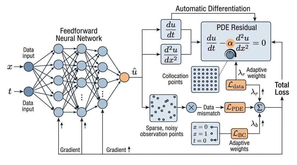
The PINN approach treats both the solution \(u(x, t)\) and the unknown parameter \(\alpha\) as optimization targets. The network \(\hat{u}_\theta(x, t)\) approximates the temperature field, while \(\alpha\) is an additional trainable parameter. The total loss function combines three terms. Figure 50.2.1 illustrates PINN inverse problem architecture.
where:
$$\mathcal{L}_{\text{data}} = \frac{1}{N} \sum_{i=1}^{N} \left| \hat{u}_\theta(x_i, t_i) - u_i \right|^2$$ $$\mathcal{L}_{\text{PDE}} = \frac{1}{M} \sum_{j=1}^{M} \left| \frac{\partial \hat{u}_\theta}{\partial t}(x_j, t_j) - \alpha \frac{\partial^2 \hat{u}_\theta}{\partial x^2}(x_j, t_j) \right|^2$$The PDE residual is evaluated at collocation points \((x_j, t_j)\) sampled throughout the domain. These points do not require data; the PDE itself provides the supervision signal. Automatic differentiation (covered in Chapter 42) computes the required partial derivatives \(\partial \hat{u}/\partial t\) and \(\partial^2 \hat{u}/\partial x^2\) exactly through the network. In short: the PDE does not just constrain the answer; it teaches the network everywhere the data cannot reach. The diagram in Figure 50.2a below illustrates this architecture.
In a standard supervised learning problem, the supervision signal comes only from labeled data points. In a PINN, the PDE provides an additional supervision signal at every point in the domain, not just where data is available. This is why PINNs can solve inverse problems from remarkably sparse data: 50 scattered temperature measurements can suffice to recover \(\alpha\) when the heat equation provides millions of collocation-point constraints. The PDE acts as an infinitely dense regularizer that restricts the network to solutions consistent with the known physics.
2. Inverse Heat Equation with DeepXDE
DeepXDE provides a high-level API for both forward and inverse PINN problems. The following code recovers the thermal diffusivity \(\alpha\) from sparse temperature measurements using the inverse heat equation.
import deepxde as dde
import numpy as np

# True diffusivity (what we want to recover)
alpha_true = 0.4

# Define the computational domain: x in [0, 1], t in [0, 1]
geom = dde.geometry.Interval(0, 1)
timedomain = dde.geometry.TimeDomain(0, 1)
geomtime = dde.geometry.GeometryXTime(geom, timedomain)

# The unknown parameter: initialized far from the true value
alpha = dde.Variable(1.0)  # trainable scalar

# Define the PDE residual
def heat_equation(x, u):
    """PDE residual: du/dt - alpha * d2u/dx2 = 0"""
    du_t = dde.grad.jacobian(u, x, i=0, j=1)   # du/dt
    du_xx = dde.grad.hessian(u, x, i=0, j=0)    # d2u/dx2
    return du_t - alpha * du_xx

# Exact solution for generating observation data
def exact_solution(x):
    """u(x,t) = sin(pi*x) * exp(-alpha_true * pi^2 * t)"""
    return np.sin(np.pi * x[:, 0:1]) * np.exp(
        -alpha_true * np.pi**2 * x[:, 1:2]
    )

# Boundary conditions: u(0,t) = u(1,t) = 0
bc = dde.icbc.DirichletBC(
    geomtime, lambda x: 0, lambda _, on_boundary: on_boundary
)

# Initial condition: u(x,0) = sin(pi*x)
ic = dde.icbc.IC(
    geomtime,
    lambda x: np.sin(np.pi * x[:, 0:1]),
    lambda _, on_initial: on_initial,
)

# Sparse observation data (simulating sensor measurements)
n_observations = 50
rng = np.random.default_rng(42)
observe_x = rng.uniform(0.1, 0.9, (n_observations, 1))
observe_t = rng.uniform(0.1, 0.9, (n_observations, 1))
observe_pts = np.hstack([observe_x, observe_t])
observe_u = exact_solution(observe_pts)

# Add 2% Gaussian noise to observations
observe_u += 0.02 * rng.standard_normal(observe_u.shape)

# PointSetBC enforces data matching at observation points
observe_bc = dde.icbc.PointSetBC(observe_pts, observe_u, component=0)
# Assemble the PDE problem
data = dde.data.TimePDE(
    geomtime,
    heat_equation,
    [bc, ic, observe_bc],
    num_domain=2000,     # collocation points for PDE residual
    num_boundary=100,
    num_initial=100,
    num_test=500,
)

# Network architecture: 2 inputs (x, t) -> 1 output (u)
net = dde.nn.FNN(
    layer_sizes=[2, 64, 64, 64, 1],
    activation="tanh",
    kernel_initializer="Glorot normal",
)

# Build and train the model
model = dde.Model(data, net)

# Phase 1: Adam optimizer for broad convergence
model.compile(
    "adam",
    lr=1e-3,
    external_trainable_variables=[alpha],
)
losshistory, train_state = model.train(
    iterations=10000,
    display_every=2000,
)

# Phase 2: L-BFGS (a quasi-Newton optimizer that approximates
# curvature for faster convergence) for fine-tuning
model.compile(
    "L-BFGS",
    external_trainable_variables=[alpha],
)
losshistory, train_state = model.train()

# Check recovered parameter
alpha_recovered = alpha.numpy()
print(f"True alpha:      {alpha_true:.4f}")
print(f"Recovered alpha: {alpha_recovered:.4f}")
print(f"Relative error:  {abs(alpha_recovered - alpha_true) / alpha_true:.2%}")
On this problem, the two-phase training strategy (Adam for 10,000 iterations followed by L-BFGS for fine-tuning) typically recovers \(\alpha\) with relative error below 1%, even with 2% observation noise and only 50 measurement points. The key is that 2,000 collocation points enforce the heat equation throughout the domain, providing orders of magnitude more supervision than the 50 data points alone. (Fifty noisy measurements plus one known PDE outperform thousands of label-only data points, because every collocation point is a free physics lesson.)
A thermal engineer places 20 thermocouples on a composite panel and heats one edge. The recorded temperature histories contain the information needed to recover the panel's thermal diffusivity, which varies spatially due to internal defects. By modeling \(\alpha(x, y)\) as a second neural network and using the 2D heat equation as the physics constraint, a PINN can produce a spatial map of thermal diffusivity, effectively performing nondestructive evaluation. This technique has been validated experimentally by Cai et al. (2021) on carbon fiber composites, recovering diffusivity maps that agree with ultrasonic measurements to within 5%.
3. Inverse PINNs in JAX
DeepXDE provides convenience, but understanding the mechanics requires seeing the raw computation. Here is the same inverse problem implemented directly in JAX, exposing every gradient computation.
import jax
import jax.numpy as jnp
from jax import random, grad, jit, vmap
import optax

def init_network(key, layer_sizes):
    """Initialize a simple feedforward network."""
    params = []
    for in_dim, out_dim in zip(layer_sizes[:-1], layer_sizes[1:]):
        key, subkey = random.split(key)
        w = random.normal(subkey, (in_dim, out_dim)) * jnp.sqrt(2.0 / in_dim)
        key, subkey = random.split(key)
        b = jnp.zeros(out_dim)
        params.append((w, b))
    return params

def forward(params, x, t):
    """Network forward pass: (x, t) -> u."""
    h = jnp.stack([x, t], axis=-1)
    for w, b in params[:-1]:
        h = jnp.tanh(h @ w + b)
    w, b = params[-1]
    return (h @ w + b).squeeze(-1)

def pde_residual(params, alpha, x, t):
    """Compute du/dt - alpha * d2u/dx2 at a single point."""
    u_fn = lambda x_, t_: forward(params, x_, t_)

    # First derivatives
    du_dt = grad(u_fn, argnums=1)(x, t)

    # Second derivative w.r.t. x
    du_dx = grad(u_fn, argnums=0)
    d2u_dx2 = grad(du_dx, argnums=0)(x, t)

    return du_dt - alpha * d2u_dx2

# Vectorize over batches of points
pde_residual_batch = vmap(pde_residual, in_axes=(None, None, 0, 0))

@jit
def loss_fn(params, log_alpha, x_data, t_data, u_data,
            x_colloc, t_colloc, x_bc, t_bc):
    """Total PINN loss: data + PDE residual + boundary."""
    alpha = jnp.exp(log_alpha)  # ensure positivity

    # Data loss
    u_pred = vmap(forward, in_axes=(None, 0, 0))(params, x_data, t_data)
    loss_data = jnp.mean((u_pred - u_data)**2)

    # PDE residual loss
    residuals = pde_residual_batch(params, alpha, x_colloc, t_colloc)
    loss_pde = jnp.mean(residuals**2)

    # Boundary loss (u = 0 at x=0 and x=1)
    u_bc = vmap(forward, in_axes=(None, 0, 0))(params, x_bc, t_bc)
    loss_bc = jnp.mean(u_bc**2)

    return loss_data + 10.0 * loss_pde + 10.0 * loss_bc

# Training loop
key = random.PRNGKey(0)
params = init_network(key, [2, 64, 64, 64, 1])
log_alpha = jnp.log(jnp.array(1.0))  # initial guess

optimizer = optax.adam(1e-3)
opt_state = optimizer.init((params, log_alpha))

grad_fn = jit(grad(loss_fn, argnums=(0, 1)))

for step in range(10000):
    grads = grad_fn(
        params, log_alpha,
        x_data, t_data, u_data,
        x_colloc, t_colloc, x_bc, t_bc,
    )
    updates, opt_state = optimizer.update(grads, opt_state)
    params, log_alpha = optax.apply_updates((params, log_alpha), updates)

    if step % 2000 == 0:
        alpha_est = float(jnp.exp(log_alpha))
        print(f"Step {step:5d} | alpha = {alpha_est:.4f}")

print(f"\nRecovered alpha: {float(jnp.exp(log_alpha)):.4f}")
print(f"True alpha:      {alpha_true:.4f}")
The JAX implementation makes several design choices visible. We parameterize \(\alpha\)
as \(\exp(\log \alpha)\) to enforce positivity without constrained optimization. The
vmap transform vectorizes the per-point PDE residual over the collocation
batch. And grad computes the exact derivatives \(\partial u / \partial t\)
and \(\partial^2 u / \partial x^2\) through the network, with no finite differences
and no discretization error.
The JAX implementation above requires about 80 lines of code for what DeepXDE accomplishes in 20 lines. DeepXDE handles domain geometry, collocation point sampling, boundary/initial condition enforcement, multi-phase training, and result visualization automatically. Use the JAX approach when you need custom loss terms, unusual architectures, or integration with other JAX-based pipelines. Use DeepXDE when the problem fits its supported PDE types and you want rapid prototyping.
4. Noether's Theorem as a Structural Prior
Recovering unknown coefficients is only half the story; we can also embed the fundamental symmetries of physics directly into the network architecture, so the model cannot produce solutions that violate conservation laws in the first place.
Noether's theorem is one of the deepest results in theoretical physics: every continuous symmetry of a physical system corresponds to a conserved quantity. Time-translation symmetry gives conservation of energy. Spatial-translation symmetry gives conservation of momentum. Rotational symmetry gives conservation of angular momentum. For discovery AI, Noether's theorem provides structural priors that constrain the space of possible physical laws.
The connection to machine learning is through Lagrangian and Hamiltonian neural networks. Instead of learning the dynamics \(\dot{x} = f(x)\) directly, we learn the Lagrangian \(L(q, \dot{q})\) or Hamiltonian \(H(q, p)\), and derive the dynamics through the Euler-Lagrange or Hamilton's equations (variational and symplectic formulations that express a system's time evolution purely in terms of energy functions rather than forces). This architectural choice automatically ensures energy conservation, because the Hamiltonian is a constant of motion by construction.
import jax
import jax.numpy as jnp
from jax import grad, jit, vmap

def hamiltonian_nn(params, q, p):
    """
    Neural network that outputs a scalar Hamiltonian H(q, p).
    The dynamics are derived from Hamilton's equations:
        dq/dt =  dH/dp
        dp/dt = -dH/dq
    """
    x = jnp.concatenate([q, p])
    for w, b in params[:-1]:
        x = jnp.tanh(x @ w + b)
    w, b = params[-1]
    H = (x @ w + b).squeeze()
    return H

def hamiltonian_dynamics(params, q, p):
    """
    Derive equations of motion from the Hamiltonian.
    Energy conservation is guaranteed by construction.
    """
    dH_dq = grad(hamiltonian_nn, argnums=1)(params, q, p)
    dH_dp = grad(hamiltonian_nn, argnums=2)(params, q, p)

    dq_dt = dH_dp    # Hamilton's first equation
    dp_dt = -dH_dq   # Hamilton's second equation

    return dq_dt, dp_dt

def rollout(params, q0, p0, dt, n_steps):
    """Symplectic Euler integration (a structure-preserving integrator
    that updates momentum and position in sequence to conserve energy
    over long time horizons) preserving Hamiltonian structure."""
    q, p = q0, p0
    trajectory = [(q, p)]

    for _ in range(n_steps):
        dq, dp = hamiltonian_dynamics(params, q, p)
        p = p + dp * dt      # update momentum first
        dq, _ = hamiltonian_dynamics(params, q, p)
        q = q + dq * dt      # then update position
        trajectory.append((q, p))

    return trajectory
Mental Model
Think of Noether's theorem like double-entry bookkeeping in accounting. Every legitimate transaction (symmetry) forces two ledger entries that must balance (conserved quantity). You cannot record revenue without a corresponding asset change; the structure of the bookkeeping system makes embezzlement visible, not a rule that someone checks after the fact. Similarly, a Hamiltonian neural network does not add a penalty that says "please conserve energy"; the architecture itself forces every change in position to be balanced by a corresponding change in momentum, so energy conservation is a structural guarantee rather than an aspirational loss term. Just as double-entry bookkeeping catches errors that a single-column ledger would miss, the Hamiltonian architecture catches unphysical trajectories that a generic neural ODE would silently produce.
The Hamiltonian Neural Network (HNN) of Greydanus et al. (2019) preserves energy by construction (up to integration error), producing closed orbits that match the true physics over thousands of time steps. A standard neural ODE (where a neural network directly parameterizes the time derivative \(\dot{x} = f_\theta(x)\) without any structural physics constraint), by contrast, drifts in energy and spirals into unphysical trajectories.
Noether's theorem tells us what to conserve; Hamiltonian/Lagrangian network architectures tell us how to conserve it. The pattern generalizes beyond energy: if you know your system conserves momentum, angular momentum, or any other quantity, you can design network architectures that preserve those quantities by construction. This is fundamentally different from adding a conservation penalty to the loss function (which is approximate and can be violated during training). Architectural constraints are exact and cannot be violated regardless of the training procedure.
5. Simulation-Based Inference
Not every inverse problem in physics has a tractable likelihood function. Many settings provide a forward simulator (particle physics Monte Carlo, cosmological N-body simulation, climate model) that maps parameters \(\theta\) to observables \(x\). Yet evaluating \(p(x | \theta)\) analytically is impossible. Simulation-based inference (SBI) addresses this by learning the posterior \(p(\theta | x)\) directly from simulated parameter-observation pairs.
The Three Main SBI Approaches
Neural Posterior Estimation (NPE) trains a conditional density estimator (typically a normalizing flow) to approximate \(p(\theta | x)\) from simulated pairs \(\{(\theta_i, x_i)\}\). Given a new observation \(x_{\text{obs}}\), the trained network immediately produces the posterior without additional simulations.
Neural Likelihood Estimation (NLE) learns \(p(x | \theta)\) instead, then combines with a prior via Bayes' rule. This is useful when the prior changes between analyses but the likelihood does not.
Neural Ratio Estimation (NRE) learns the likelihood-to-evidence ratio \(r(x, \theta) = p(x | \theta) / p(x)\) using a binary classifier, avoiding explicit density estimation entirely.
Checkpoint
So far: all three SBI approaches (NPE, NLE, NRE) bypass an intractable likelihood by training neural networks on simulated parameter-observation pairs, but they differ in what they learn (the posterior, the likelihood, or the likelihood-to-evidence ratio) and therefore in when each is most convenient.
import torch
import numpy as np

# Example: inferring parameters of a damped oscillator
# from noisy trajectory observations

def simulator(theta):
    """
    Forward simulator: damped oscillator.
    theta = [amplitude, damping, frequency]
    Returns a noisy trajectory (100 time points).
    """
    A, gamma, omega = theta
    t = np.linspace(0, 10, 100)
    x = A * np.exp(-gamma * t) * np.cos(omega * t)
    # Add observation noise
    x += 0.05 * np.random.randn(len(t))
    return x

def generate_training_data(n_simulations=10000):
    """Generate parameter-observation pairs for SBI training."""
    prior_low = np.array([0.5, 0.1, 1.0])
    prior_high = np.array([3.0, 1.0, 8.0])

    thetas = np.random.uniform(prior_low, prior_high,
                                size=(n_simulations, 3))
    observations = np.array([simulator(theta) for theta in thetas])

    return (
        torch.tensor(thetas, dtype=torch.float32),
        torch.tensor(observations, dtype=torch.float32),
    )

# Using the sbi library for Neural Posterior Estimation
# (sbi v0.22+; earlier versions used a slightly different API)
from sbi.inference import SNPE
from sbi.utils import BoxUniform

# Define prior
prior = BoxUniform(
    low=torch.tensor([0.5, 0.1, 1.0]),
    high=torch.tensor([3.0, 1.0, 8.0]),
)

# Generate training simulations
thetas, observations = generate_training_data(10000)

# Train the neural posterior estimator
inference = SNPE(prior=prior)
inference.append_simulations(thetas, observations)
density_estimator = inference.train()

# Build the posterior
posterior = inference.build_posterior(density_estimator)

# Given a real observation, sample from the posterior
x_observed = torch.tensor(simulator([2.0, 0.3, 4.0]),
                           dtype=torch.float32)
samples = posterior.sample((5000,), x=x_observed)

print(f"Posterior mean: {samples.mean(dim=0).numpy()}")
print(f"Posterior std:  {samples.std(dim=0).numpy()}")
print(f"True values:    [2.0, 0.3, 4.0]")
sbi library (v0.23+) has refactored its API to unify inference classes; check the current documentation if method signatures differ from this example.The SBI approach is particularly powerful for physics problems where the forward model is expensive (each simulation takes minutes to hours) but we need to perform inference for many different observations. Once the density estimator is trained, posterior evaluation is instantaneous, amortizing the cost of the training simulations across all future inferences.
The Laser Interferometer Gravitational-Wave Observatory (LIGO)/Virgo collaboration detects gravitational waves from merging black holes and neutron stars. Inferring the source parameters (masses, spins, distance, sky location) from the detected signal traditionally requires running Markov Chain Monte Carlo (MCMC) samplers for hours per event. The DINGO system (Dax et al., 2021) trains a normalizing flow on millions of simulated gravitational waveforms, then produces posterior samples for a new event in under one second (circa 2021). The authors reported roughly a 1000x speedup over traditional MCMC, enabling real-time alerts for electromagnetic follow-up observations. As of 2024, DINGO-IS (Dax et al., 2023) extends this approach with importance sampling to provide asymptotically exact posteriors, and flow-matching architectures are increasingly replacing normalizing flows for amortized SBI in gravitational-wave astronomy.
6. Failure Modes and Mitigations
The power of PINNs and SBI comes with practical pitfalls that can silently undermine results if left unaddressed.
PINNs are not a universal solution. Several well-documented failure modes require awareness and mitigation strategies.
Spectral bias. Neural networks with smooth activation functions learn low-frequency components of the solution first, struggling with sharp gradients, shocks, and high-frequency oscillations. For the Burgers equation with viscosity approaching zero, standard PINNs tend to fail severely. Mitigation: use Fourier feature embeddings (Tancik et al., 2020) or multi-scale architectures that explicitly represent high-frequency content.
Imbalanced loss terms. The data loss, PDE residual, and boundary losses operate on different scales. If the PDE residual dominates, the network satisfies the equation approximately but ignores the data. If the data loss dominates, the network interpolates the data but violates the physics between measurement points. Mitigation: use adaptive loss weighting (Wang et al., 2021) or the neural tangent kernel perspective (a theoretical framework that analyzes neural network training dynamics through the lens of kernel methods, revealing how different loss components compete for gradient updates) to balance gradient magnitudes across loss terms.
Common Misconception
A frequent misconception is that adding more collocation points (where the PDE residual is evaluated) will always improve PINN accuracy, analogous to how more training data helps in standard supervised learning. In practice, increasing collocation points beyond a moderate number often degrades performance because it amplifies the PDE residual loss relative to the data and boundary losses, creating a severe imbalance that causes the optimizer to satisfy the equation in a vacuum while ignoring the observations. The dominant factor for PINN accuracy is proper loss balancing across terms, not the raw number of collocation points.
Optimization landscape. The composite loss function can have many local minima, saddle points, and flat regions. The two-phase training strategy (Adam followed by L-BFGS) helps but does not guarantee convergence to the global minimum. Mitigation: use curriculum training (start with easier sub-problems), causal training (enforce temporal causality), or ensemble methods to explore the loss landscape more thoroughly.
# Adaptive loss weighting (Learning Rate Annealing)
# following Wang et al. (2021)

def adaptive_weights(loss_data, loss_pde, loss_bc,
                     prev_weights, eta=0.1):
    """
    Update loss weights based on gradient statistics.
    Balances gradient magnitudes across loss components.
    """
    # Compute gradient norms for each loss term
    grad_data = jax.grad(lambda p: loss_data(p))(params)
    grad_pde = jax.grad(lambda p: loss_pde(p))(params)
    grad_bc = jax.grad(lambda p: loss_bc(p))(params)

    norm_data = jnp.sqrt(sum(
        jnp.sum(g**2) for g in jax.tree_util.tree_leaves(grad_data)
    ))
    norm_pde = jnp.sqrt(sum(
        jnp.sum(g**2) for g in jax.tree_util.tree_leaves(grad_pde)
    ))
    norm_bc = jnp.sqrt(sum(
        jnp.sum(g**2) for g in jax.tree_util.tree_leaves(grad_bc)
    ))

    # Target: equal gradient contributions
    max_norm = jnp.maximum(norm_data, jnp.maximum(norm_pde, norm_bc))
    w_data = max_norm / (norm_data + 1e-8)
    w_pde = max_norm / (norm_pde + 1e-8)
    w_bc = max_norm / (norm_bc + 1e-8)

    # Exponential moving average for stability
    w_data = (1 - eta) * prev_weights[0] + eta * w_data
    w_pde = (1 - eta) * prev_weights[1] + eta * w_pde
    w_bc = (1 - eta) * prev_weights[2] + eta * w_bc

    return jnp.array([w_data, w_pde, w_bc])
7. When to Use Each Approach
The choice between PINNs, SBI, and classical inverse methods depends on the problem structure:
| Criterion | Classical (MCMC) | PINN Inverse | SBI |
|---|---|---|---|
| Likelihood tractable? | Required | Not needed | Not needed |
| PDE known? | Often yes | Required | Simulator only |
| Posterior uncertainty? | Yes | Limited | Yes |
| Amortized inference? (train once, then obtain posteriors for new observations instantly without retraining) | No | No | Yes |
| Cost per new observation | High | Moderate | Low |
| Best for | Well-posed, moderate-dim | PDE parameter recovery | Expensive simulators |
For physics discovery, PINNs and SBI are complementary rather than competing. PINNs excel when the governing PDE is known and the unknown is a small number of parameters. SBI excels when the forward model is a complex simulator and you need full posterior uncertainty quantification. In Section 50.4, we combine both: PySR discovers the equation form, a PINN recovers unknown coefficients, and Bayesian optimization explores the design space.
Research Frontier
Hao et al. (2023) introduced PINNacle, a comprehensive benchmark suite that systematically evaluates PINNs across 20 diverse PDE problems spanning diffusion, reaction-diffusion, incompressible flow, compressible flow, and solid mechanics. The benchmark revealed that no single PINN variant dominates all problem classes, and that techniques such as causal training (Respecting Causality, Wang et al., 2022) and separable PINNs (Cho et al., 2024) can close much of the gap between PINNs and classical solvers on stiff, multi-scale, and chaotic systems. PINNacle also exposed that reported accuracies in the literature are often not reproducible under controlled hyperparameter budgets, motivating standardized evaluation protocols for physics-informed methods.
Try It: Recover a Spring Constant with a PINN
Build a minimal inverse PINN that recovers the spring constant \(k\) of a damped harmonic oscillator from noisy position measurements. This project requires only PyTorch (or JAX) and NumPy.
Step 1. Generate synthetic data: simulate
\(\ddot{x} + 0.1\dot{x} + k\,x = 0\) with \(k = 4.0\), \(x(0) = 1\), \(\dot{x}(0) = 0\)
using scipy.integrate.solve_ivp to produce 200 time points over
\(t \in [0, 10]\). Add 3% Gaussian noise to the position values.
Step 2. Subsample 30 noisy observations at random times to serve as your sparse measurement set.
Step 3. Build a small feedforward network (3 hidden layers, 32 units,
tanh activations) that takes \(t\) as input and outputs predicted position \(\hat{x}(t)\).
Define k as a trainable scalar parameter initialized to 1.0.
Step 4. Construct the PINN loss: (a) a data term matching the 30 observations, (b) a PDE residual term evaluating \(\ddot{\hat{x}} + 0.1\dot{\hat{x}} + k\,\hat{x}\) at 500 collocation points sampled uniformly in \([0, 10]\), and (c) an initial-condition term enforcing \(\hat{x}(0) = 1\) and \(\dot{\hat{x}}(0) = 0\). Use automatic differentiation for all derivatives.
Step 5. Train with Adam (learning rate \(10^{-3}\)) for 5,000 steps. Print \(k\) every 1,000 steps and verify it converges to approximately 4.0. Plot the predicted trajectory against the noisy data and the ground truth to visualize how the physics constraint fills in the gaps between sparse measurements.
Exercise 50.2.1
Suppose you set up an inverse PINN for the 1D heat equation with 50 noisy observations and 2,000 collocation points, but after training, the recovered diffusivity \(\hat{\alpha}\) has a 40% relative error. You suspect a loss imbalance. Without changing the number of collocation points or observations, describe two concrete changes to the training procedure that could fix the problem, and explain why each one works.
Hint
Look at section 6 (Failure Modes). One approach adjusts the loss weights dynamically based on gradient magnitudes. The other changes the optimization schedule (think about what the two-phase strategy does and whether your initial Adam learning rate or iteration count might be insufficient for the PDE residual to decrease enough before L-BFGS fine-tuning begins).
Step-Through: Inverse PINN Training on a 3-Point Domain
Trace one gradient step of an inverse PINN for the heat equation on a toy domain with concrete numbers. Suppose \(\alpha = 1.0\) (current estimate; true value is 0.4). Our network predicts \(\hat{u}(0.5, 0.3) = 0.71\), and the single observation there is \(u_{\text{obs}} = 0.68\). At one collocation point \((0.5, 0.3)\), autodiff gives \(\partial \hat{u}/\partial t = -1.20\) and \(\partial^2 \hat{u}/\partial x^2 = -0.95\).
Data loss: \((0.71 - 0.68)^2 = 0.0009\).
PDE residual: $r = (-1.20) - (1.0)(-0.95) = -1.20 + 0.95 = -0.25$; squared residual \(= 0.0625\). With weight \(\lambda_r = 10\), the PDE contribution is \(0.625\).
Total loss: \(0.0009 + 0.625 = 0.6259\). The PDE term dominates. Its gradient with respect to \(\alpha\) is $\partial r^2 / \partial \alpha = 2r \cdot (-\partial^2 \hat{u}/\partial x^2) = 2(-0.25)(0.95) = -0.475$. So a positive step on $\alpha$ would decrease the residual, but \(\alpha\) is already too high (1.0 vs. true 0.4), meaning the optimizer must first drive the network outputs \(\hat{u}\) toward values whose second spatial derivative better matches the observations before \(\alpha\) can descend. This illustrates why two-phase training helps: Adam reshapes \(\hat{u}\) broadly, then L-BFGS fine-tunes \(\alpha\).
Real-World Application: Subsurface Flow Characterization
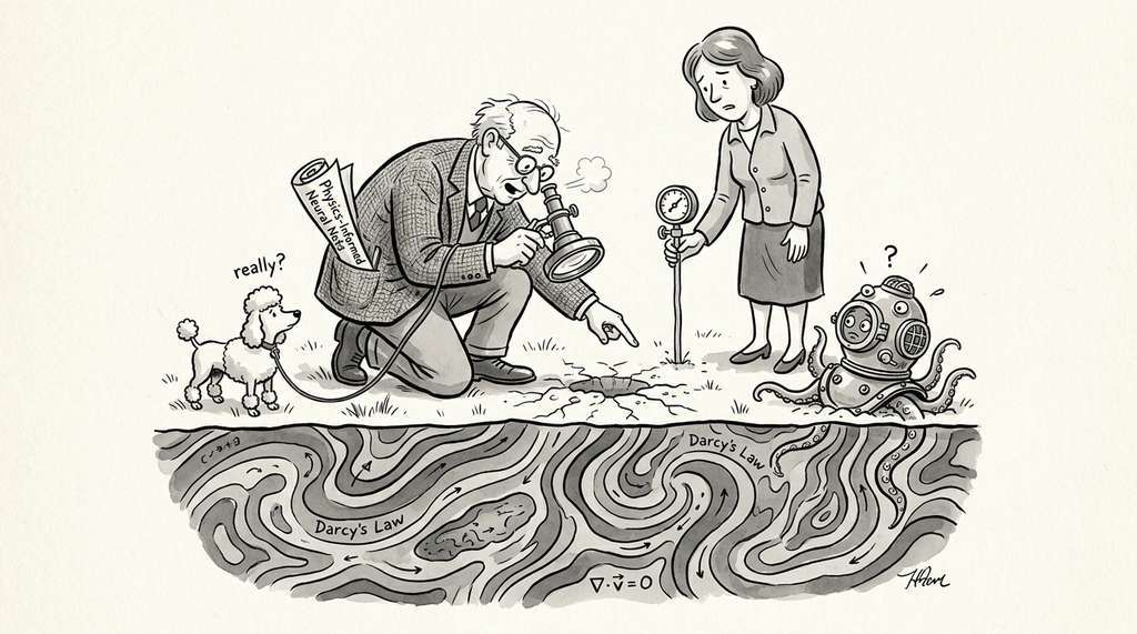
The Pacific Northwest National Laboratory uses physics-informed neural networks to infer subsurface permeability fields from sparse well-pressure measurements in groundwater aquifers. By embedding Darcy's law and the continuity equation as PDE constraints, their PINN system recovers spatially varying permeability maps from fewer than 20 monitoring wells, guiding decisions about contaminant remediation and water resource management across sites where direct core sampling would cost millions of dollars.
The Neural Network That Rediscovered Fourier
When Raissi, Perdikaris, and Karniadakis published their foundational 2019 PINN paper, they tested it on the Schrodinger equation and discovered that the network spontaneously learned to decompose the solution into real and imaginary parts that closely mirrored a truncated Fourier series, despite never being told about Fourier analysis. The network had, in effect, converged on representations resembling a truncated Fourier series, likely because the PDE loss landscape made sinusoidal basis functions a natural low-loss path. This became one of the earliest concrete examples of a neural network rediscovering classical mathematical structure purely from a physics constraint.
Lab: Recovering Thermal Diffusivity Under Increasing Noise
Goal: Measure how observation noise degrades inverse PINN accuracy and find the noise level at which recovery fails.
Tools: Python with DeepXDE (or JAX/PyTorch), NumPy, Matplotlib. Use the 1D heat equation setup from section 2.
What to vary: Run the inverse PINN six times with noise levels \(\sigma \in \{0, 0.01, 0.02, 0.05, 0.10, 0.20\}\) added to the 50 synthetic observations. Keep all other settings identical (2,000 collocation points, same network architecture, same two-phase optimizer).
What to observe: For each noise level, record the recovered \(\hat{\alpha}\), its relative error, and the final PDE residual loss. Plot relative error vs. noise level. Identify the noise threshold where relative error exceeds 5%. Then repeat the experiment with 200 observations instead of 50 at the worst noise level and check whether more data compensates for higher noise. Document whether the PDE residual loss or the data loss dominates at each noise level.
Time estimate: 20 minutes (each training run takes about 1-2 minutes on a CPU).