Prerequisites
This section builds directly on the automation infrastructure from Section 55.1 and the acquisition functions from Chapter 46. Familiarity with Gaussian processes and Bayesian optimization from Chapter 32 is essential. The discussion of LLM-based planners assumes knowledge of agent architectures from Chapter 40.
Chapter 46 built an experiment planner that selects the next experiment to maximize information gain. Section 55.1 built the automation infrastructure that executes experiments on robotic hardware. This section connects them into a single closed loop. The result is a system where no human stands between the AI's decision to "try compound X at concentration Y" and the actual measurement of compound X at concentration Y. The loop runs continuously: plan, execute, observe, update. Each cycle typically takes minutes instead of the days or weeks a human-in-the-loop workflow requires. This acceleration is the central promise of the self-driving laboratory (SDL).
1. The Four-Stage SDL Loop
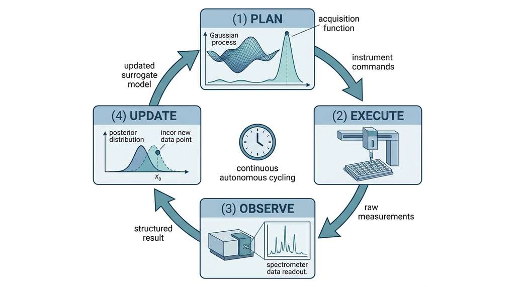
Every self-driving laboratory, regardless of scientific domain or hardware platform, implements the same four-stage loop. Figure 55.2 illustrates this cycle: the planner selects the next experiment, the executor runs it on hardware, the observer extracts a measurement, and the updater refits the surrogate model before the cycle repeats. Figure 55.2.1 illustrates Four-stage SDL closed loop.
At 2:47 AM on a Tuesday in 2023, a robotic arm in a Berkeley lab loaded a crucible into a furnace. Forty minutes later, a diffractometer measured the resulting crystal structure. A Bayesian optimizer then selected the next composition to try. Every member of the research team was asleep. By morning the system had completed eleven synthesis cycles and discovered a ternary oxide that no human had predicted. This is closed-loop experimentation: a software system autonomously decides what experiment to run next, executes it on physical or simulated hardware, measures the outcome, and feeds that measurement back into the decision model. No human intervenes between cycles. The approach compresses iteration time from days (a human reviews data, thinks, and schedules the next run) to minutes (the model updates, the acquisition function re-optimizes, and the robot acts). One weekend can yield what a traditional lab achieves in a month. The mechanism is straightforward: a surrogate model (typically a Gaussian process, or GP) maintains a probabilistic belief about the objective surface, and an acquisition function converts that belief into a score for every candidate experiment, so the system always picks the candidate with the highest expected value of information. Use closed-loop automation when the experimental cost per sample is moderate to high and the design space is continuous or combinatorial but searchable; for very cheap assays where exhaustive screening is feasible, or for problems requiring irreplaceable human judgment at each step, a simpler batch design or human-in-the-loop workflow may be more appropriate.
The Four Stages in Detail
Stage 1: Plan. The AI planner selects the next experiment(s) to run. In Bayesian optimization, this means maximizing an acquisition function (Expected Improvement (EI), Upper Confidence Bound (UCB), or Bayesian Active Learning by Disagreement (BALD) from Section 46.2) over the design space. In large language model (LLM) planning (Coscientist), the planner generates a natural-language experiment description that is parsed into structured commands. The output of this stage is a set of experiment specifications: what to synthesize, at what conditions, and what to measure.
Stage 2: Execute. The orchestration layer translates experiment specifications into instrument commands and dispatches them through the scheduler from Section 55.1. The liquid handler prepares samples, the incubator maintains temperature, and the robot arm transfers plates between stations. Execution must be idempotent (repeating the same command produces the same result without side effects) where possible: if a transfer fails midway, the system should be able to retry without corrupting the experiment.
Stage 3: Observe. Measurement instruments characterize the prepared samples and return raw data. The observation stage includes data preprocessing: background subtraction, normalization, outlier detection, and unit conversion. The output is a structured result (feature vector, scalar measurement, or spectrum) in the format the surrogate model expects.
Stage 4: Update. The surrogate model incorporates the new observation and updates its predictions. For a GP, this means conditioning on the new data point and recomputing the posterior mean and variance. For a neural network surrogate, this means a round of fine-tuning. The updated model feeds back into Stage 1, and the loop repeats. In short: A closed loop that updates its beliefs after every experiment will always outperform one that plans blind, because each observation steers the next attempt toward the optimum instead of into already-explored territory.
Mental Model
Think of the SDL loop like a chef perfecting a recipe through systematic tasting. The chef has a mental model of how ingredients interact (the surrogate model). She tastes the current dish (observe), updates her understanding of what is missing (update), decides what adjustment to try next based on what she expects will improve the dish most (plan via acquisition function), and makes the adjustment (execute). The key parallel is that each tasting changes her mental model: after learning that more salt improved the flavor but more acid did not, she concentrates future experiments in the "salt plus herbs" region rather than wasting attempts on acid. A chef who tastes after every tweak converges on a great dish far faster than one who makes ten blind changes and only tastes at the end, just as a closed-loop SDL with per-round model updates outperforms batch-mode experimentation.
Formally, let \(\mathcal{D}_t = \{(\mathbf{x}_i, y_i)\}_{i=1}^{t}\) be the dataset after \(t\) iterations, where \(\mathbf{x}_i \in \mathcal{X}\) is the experiment specification and \(y_i \in \mathbb{R}\) is the measurement. The surrogate model \(f \sim \mathcal{GP}(\mu_t, k_t)\) provides a posterior predictive distribution \(p(y \mid \mathbf{x}, \mathcal{D}_t)\) at any unobserved point \(\mathbf{x}\). The acquisition function \(\alpha_t(\mathbf{x})\) scores each candidate experiment by its expected utility (information gain, improvement probability, or upper confidence bound). The planner selects:
$$\mathbf{x}_{t+1} = \arg\max_{\mathbf{x} \in \mathcal{X}_{\text{safe}}} \alpha_t(\mathbf{x})$$where \(\mathcal{X}_{\text{safe}} \subseteq \mathcal{X}\) is the subset of the design space that satisfies safety constraints (see Section 55.3). The executor runs the experiment at \(\mathbf{x}_{t+1}\), the observer returns \(y_{t+1}\), and the updater computes \(\mathcal{D}_{t+1} = \mathcal{D}_t \cup \{(\mathbf{x}_{t+1}, y_{t+1})\}\).
Checkpoint
So far: the SDL loop has four stages (plan, execute, observe, update), each cycle selects the next experiment by maximizing an acquisition function \(\alpha_t\) over a safe design space \(\mathcal{X}_{\text{safe}}\), and the surrogate model (a GP) refits on the growing dataset \(\mathcal{D}_t\) after every observation.
The sample efficiency of Bayesian optimization depends on the surrogate model being updated before the next acquisition decision. If the update lags (because the model takes an hour to retrain, or because results are batched and delayed), the planner makes decisions based on stale information and wastes experiments. The engineering challenge is to keep the update latency below the execution latency. For a 96-well plate that takes 30 minutes to prepare and measure, the model update must complete in under 30 minutes. For high-throughput screening at thousands of compounds per day, the model must update in seconds.
2. Implementing the Loop
Keeping update latency below execution latency is ultimately an engineering problem, so the next step is to turn the four-stage abstraction into concrete, swappable software components.
The following implementation expresses the four-stage loop as composable Python components. Each stage is an abstract class with a concrete implementation for the simulated SDL.
"""The four-stage SDL loop as composable components.

Each stage is a protocol class that concrete implementations must
satisfy. The SDLLoop class orchestrates the stages and manages
the experiment history.
"""
from typing import Protocol, Any
from dataclasses import dataclass, field
import numpy as np
import time
import json


@dataclass
class ExperimentSpec:
    """Specification for a single experiment."""
    experiment_id: str
    parameters: dict[str, float]   # design variables
    metadata: dict[str, Any] = field(default_factory=dict)


@dataclass
class ExperimentResult:
    """Result of executing and observing an experiment."""
    experiment_id: str
    parameters: dict[str, float]
    observation: float             # scalar measurement
    observation_metadata: dict = field(default_factory=dict)
    timestamp: float = 0.0

    def __post_init__(self):
        if self.timestamp == 0.0:
            self.timestamp = time.time()


class Planner(Protocol):
    """Selects the next experiment(s) to run."""

    def propose(self, history: list[ExperimentResult],
                n_proposals: int) -> list[ExperimentSpec]:
        """Propose n experiments based on history."""
        ...


class Executor(Protocol):
    """Translates experiment specs into instrument commands."""

    def execute(self, spec: ExperimentSpec) -> dict:
        """Execute an experiment, return raw instrument data."""
        ...


class Observer(Protocol):
    """Extracts structured observations from raw instrument data."""

    def observe(self, spec: ExperimentSpec,
                raw_data: dict) -> float:
        """Process raw data into a scalar observation."""
        ...


class Updater(Protocol):
    """Updates the surrogate model with new observations."""

    def update(self, history: list[ExperimentResult]) -> None:
        """Refit the surrogate model on accumulated data."""
        ...


class SDLLoop:
    """Orchestrates the four-stage self-driving lab loop.

    Connects planner, executor, observer, and updater into a
    continuous experimentation cycle with full provenance logging.
    """

    def __init__(self, planner: Planner, executor: Executor,
                 observer: Observer, updater: Updater,
                 batch_size: int = 1):
        self.planner = planner
        self.executor = executor
        self.observer = observer
        self.updater = updater
        self.batch_size = batch_size
        self.history: list[ExperimentResult] = []
        self.round_log: list[dict] = []

    def run_round(self, round_number: int) -> list[ExperimentResult]:
        """Execute one complete plan-execute-observe-update cycle.

        Returns the results from this round.
        """
        round_start = time.time()

        # Stage 1: Plan
        proposals = self.planner.propose(
            self.history, n_proposals=self.batch_size
        )

        # Stages 2-3: Execute and Observe
        round_results = []
        for spec in proposals:
            raw_data = self.executor.execute(spec)
            observation = self.observer.observe(spec, raw_data)
            result = ExperimentResult(
                experiment_id=spec.experiment_id,
                parameters=spec.parameters,
                observation=observation,
                observation_metadata=raw_data
            )
            round_results.append(result)
            self.history.append(result)

        # Stage 4: Update
        self.updater.update(self.history)

        # Log the round
        self.round_log.append({
            "round": round_number,
            "n_experiments": len(round_results),
            "best_so_far": max(r.observation for r in self.history),
            "wall_time_s": time.time() - round_start
        })

        return round_results

    def run(self, n_rounds: int) -> list[ExperimentResult]:
        """Run the SDL loop for n_rounds."""
        for i in range(n_rounds):
            self.run_round(i)
        return self.history

    def summary(self) -> dict:
        """Return a summary of the SDL campaign."""
        if not self.history:
            return {"status": "no experiments run"}
        observations = [r.observation for r in self.history]
        return {
            "total_experiments": len(self.history),
            "n_rounds": len(self.round_log),
            "best_observation": max(observations),
            "mean_observation": np.mean(observations),
            "best_parameters": max(
                self.history, key=lambda r: r.observation
            ).parameters
        }
SDLLoop orchestrator connects any planner, executor, observer, and updater into a closed-loop experimentation cycle. Each round logs provenance metadata (wall time, best-so-far) for the experiment registry.The Protocol-based design (Python's structural subtyping mechanism, where any class that implements the required methods satisfies the interface without explicit inheritance) in Listing 55.5 decouples the loop logic from any specific planner or instrument. You can swap a Bayesian optimization planner for an LLM-based planner, or replace the simulated executor with a real instrument adapter, without changing the loop code. This composability is essential for production SDLs that evolve their hardware and algorithms over time.
With the composable loop in hand, the natural question is how production systems have implemented each stage in practice.
3. Reference Architectures
Three published SDL architectures illustrate different points in the design space. Understanding their trade-offs helps you choose the right architecture for your own SDL.
3.1 ChemOS 2.0: Modular Orchestration
ChemOS 2.0 (Roch et al., 2022) is an orchestration platform for chemical self-driving laboratories. Its architecture separates concerns into five modules: a Planner (Bayesian optimization via Phoenics, a kernel-density-based Bayesian optimizer designed for small-data chemistry campaigns), a Chemist (translates abstract synthesis plans into instrument-specific protocols), an Executor (dispatches to robotic hardware via vendor APIs), an Analyst (processes raw instrument data into structured observations), and a Manager (coordinates the other modules and manages the experiment queue).
ChemOS 2.0's key contribution is the separation between the Chemist (domain translation) and the Executor (hardware abstraction). The Chemist knows chemistry: it understands that "synthesize compound X" requires dissolving precursors, adding reagents in a specific order, and maintaining temperature control. The Executor knows hardware: it translates "maintain 80C for 2 hours" into heater control commands. This separation means a new synthesis protocol only requires updating the Chemist module, not the hardware layer.
3.2 Coscientist: LLM-Driven Planning
Coscientist (Boiko et al., 2023) replaces the Bayesian optimization planner with an LLM (GPT-4) that reasons about chemistry in natural language. Given a goal ("optimize the yield of a Suzuki coupling reaction"), the LLM generates a hypothesis ("increasing the catalyst loading from 2 mol% to 5 mol% should increase yield"), translates it into an executable experiment plan (specific reagent volumes, temperatures, and times), and dispatches the plan to a robotic platform (Opentrons OT-2; as of 2024, the Opentrons Flex has become the preferred platform for new SDL installations, offering a larger deck and more flexible pipetting capabilities).
The LLM-based approach offers three advantages over Bayesian optimization. First, it can incorporate qualitative chemical knowledge ("palladium catalysts are sensitive to moisture") that a GP kernel cannot easily encode. Second, it generates human-readable experiment rationales, improving interpretability. Third, it can handle multi-step synthesis protocols where each step's outcome affects the next. Standard BO struggles in this setting because the design space is combinatorial and step-dependent.
The disadvantage is reliability: the LLM sometimes generates chemically invalid protocols (impossible reagent combinations, unsafe conditions) that a Bayesian optimizer constrained to a validated design space would never propose. This motivates the safety layer in Section 55.3.
"""LLM-based experiment planner following the Coscientist pattern.

Uses structured prompting to generate experiment specifications
from natural language goals, with schema validation.
"""
from dataclasses import dataclass
import json
import re


@dataclass
class LLMPlannerConfig:
    """Configuration for an LLM-based experiment planner."""
    design_space: dict[str, tuple[float, float]]  # param -> (min, max)
    objective_description: str
    constraints: list[str] = None

    def __post_init__(self):
        if self.constraints is None:
            self.constraints = []


class LLMExperimentPlanner:
    """Planner that uses structured LLM output for experiment design.

    In production, this calls an LLM API. Here we demonstrate the
    prompt template and output parsing that connect the LLM to the
    SDL loop.
    """

    PROMPT_TEMPLATE = """You are a chemistry experiment planner for a
self-driving laboratory. Your goal: {objective}

Design space (parameter name -> [min, max]):
{design_space}

Safety constraints:
{constraints}

Previous experiments and results:
{history}

Propose {n_proposals} new experiment(s) as JSON. Each experiment
must have a "parameters" dict with values within the design space
bounds. Include a "rationale" field explaining your reasoning.

Output format:
[{{"parameters": {{"param1": value, ...}}, "rationale": "..."}}]
"""

    def __init__(self, config: LLMPlannerConfig):
        self.config = config

    def build_prompt(self, history: list[ExperimentResult],
                     n_proposals: int) -> str:
        """Construct the planning prompt from history and config."""
        ds_str = "\n".join(
            f"  {name}: [{lo}, {hi}]"
            for name, (lo, hi) in self.config.design_space.items()
        )
        constraints_str = "\n".join(
            f"  - {c}" for c in self.config.constraints
        ) or "  None"
        history_str = "\n".join(
            f"  Exp {r.experiment_id}: params={r.parameters}, "
            f"result={r.observation:.4f}"
            for r in history[-10:]  # last 10 for context window
        ) or "  No previous experiments"

        return self.PROMPT_TEMPLATE.format(
            objective=self.config.objective_description,
            design_space=ds_str,
            constraints=constraints_str,
            history=history_str,
            n_proposals=n_proposals
        )

    def parse_response(self, response_text: str,
                       round_id: int) -> list[ExperimentSpec]:
        """Parse LLM response into validated ExperimentSpec objects."""
        # Extract JSON from response (handle markdown code blocks)
        json_match = re.search(r'\[.*\]', response_text, re.DOTALL)
        if not json_match:
            raise ValueError("No JSON array found in LLM response")

        proposals = json.loads(json_match.group())
        specs = []
        for i, proposal in enumerate(proposals):
            params = proposal["parameters"]
            # Validate bounds
            for name, value in params.items():
                lo, hi = self.config.design_space[name]
                if not (lo <= value <= hi):
                    raise ValueError(
                        f"Parameter {name}={value} outside bounds "
                        f"[{lo}, {hi}]"
                    )
            specs.append(ExperimentSpec(
                experiment_id=f"round{round_id}_exp{i}",
                parameters=params,
                metadata={"rationale": proposal.get("rationale", "")}
            ))
        return specs


# Demonstrate prompt construction
config = LLMPlannerConfig(
    design_space={
        "catalyst_loading_mol_pct": (0.5, 10.0),
        "temperature_C": (25.0, 120.0),
        "reaction_time_h": (0.5, 24.0),
        "solvent_ratio": (0.0, 1.0)
    },
    objective_description=(
        "Maximize yield of Suzuki coupling reaction "
        "between aryl bromide and phenylboronic acid"
    ),
    constraints=[
        "Temperature must not exceed 120 C (solvent boiling point)",
        "Catalyst loading below 2 mol% may give incomplete conversion"
    ]
)

planner = LLMExperimentPlanner(config)
prompt = planner.build_prompt(history=[], n_proposals=2)
print(prompt[:500])  # Show first 500 chars of the prompt

# Simulate parsing an LLM response
mock_response = """Based on literature precedent for Suzuki couplings:
[
  {"parameters": {"catalyst_loading_mol_pct": 5.0,
                   "temperature_C": 80.0,
                   "reaction_time_h": 4.0,
                   "solvent_ratio": 0.5},
   "rationale": "Standard conditions from Miyaura 1995"},
  {"parameters": {"catalyst_loading_mol_pct": 3.0,
                   "temperature_C": 100.0,
                   "reaction_time_h": 2.0,
                   "solvent_ratio": 0.7},
   "rationale": "Higher temperature may compensate for lower catalyst"}
]"""

specs = planner.parse_response(mock_response, round_id=0)
for spec in specs:
    print(f"\n{spec.experiment_id}:")
    print(f"  Parameters: {spec.parameters}")
    print(f"  Rationale: {spec.metadata['rationale']}")
ExperimentSpec objects. In production, the build_prompt output goes to an LLM API; here we demonstrate the integration pattern with a mock response.3.3 GNoME to A-Lab: Prediction to Synthesis
The most striking SDL demonstration of 2023 was the pipeline from Google DeepMind's GNoME (Graph Networks for Materials Exploration) to Berkeley Lab's A-Lab. GNoME, a graph neural network trained on the Materials Project database, predicted 2.2 million thermodynamically stable crystal structures. Of these, 381,000 matched experimentally known structures, validating the model's predictions. The A-Lab then autonomously synthesized 41 of the novel GNoME-predicted materials over 17 days, achieving a 71% success rate with zero human intervention. (That is 2.2 million computational candidates distilled to 41 physical syntheses in 17 days, with no human touching a single sample.)
This pipeline illustrates a two-stage SDL architecture. The first stage is computational screening: GNoME screens a vast combinatorial space of possible crystal structures using learned energy predictions, filtering billions of candidates down to millions of stable predictions. The second stage is robotic synthesis: A-Lab takes the filtered candidates, generates synthesis recipes (precursor selection, mixing ratios, heating profiles), executes them on robotic equipment (ball mills, furnaces, X-ray diffraction (XRD) instruments), and characterizes the results.
The handoff between GNoME and A-Lab requires translating between two fundamentally different representations. GNoME outputs a crystal structure (composition, space group and lattice parameters, which specify the symmetry and dimensions of the repeating unit cell), but A-Lab needs a synthesis recipe: precursor chemicals, stoichiometric ratios, processing temperatures, and hold times. A-Lab bridges this gap with literature mining (which precursors have been used for similar compositions?) and thermodynamic reasoning (at what temperature will the precursors decompose into the target phase?).
When A-Lab receives a target composition like BaZrS\(_3\) (barium zirconium sulfide), its decision engine must choose precursors (BaCO\(_3\) + ZrO\(_2\) + S, or BaS + ZrS\(_2\)?), a synthesis method (solid-state, solution, or mechanochemical?), and processing conditions (temperature, time, atmosphere). The engine queries a database of known synthesis routes for chemically similar compounds, ranks candidates by predicted success probability (a classifier trained on prior A-Lab experiments), and generates a complete protocol. If the first attempt fails (XRD shows wrong phase), the engine adjusts conditions and retries with a modified recipe. This closed-loop retry strategy accounts for much of A-Lab's 71% success rate: many of the successful syntheses required 2-3 iterations.
4. Bayesian Optimization as the SDL Planner
Bayesian optimization (BO) is the most common planning algorithm for SDLs, covered in detail in Chapter 45 and Chapter 46. The following BO-based planner plugs directly into the SDL loop from Listing 55.5.
"""Bayesian optimization planner for the SDL loop.

Uses a Gaussian process surrogate with Expected Improvement
acquisition, implemented via BoTorch (Meta's library for Bayesian optimization
built on GPyTorch and PyTorch).
"""
import torch
import numpy as np
from botorch.models import SingleTaskGP
from botorch.fit import fit_gpytorch_mll
from botorch.acquisition import ExpectedImprovement
from botorch.optim import optimize_acqf
from gpytorch.mlls import ExactMarginalLogLikelihood


class BOPlanner:
    """Bayesian optimization planner using BoTorch.

    Fits a GP surrogate to the experiment history and proposes
    new experiments by maximizing Expected Improvement.
    """

    def __init__(self, bounds: torch.Tensor,
                 param_names: list[str]):
        """
        Args:
            bounds: (2, d) tensor of [lower, upper] bounds
            param_names: names of the d design parameters
        """
        self.bounds = bounds
        self.param_names = param_names
        self.model = None

    def propose(self, history: list[ExperimentResult],
                n_proposals: int = 1) -> list[ExperimentSpec]:
        """Propose experiments using Expected Improvement."""
        if len(history) < 2:
            # Not enough data for GP; use random proposals
            return self._random_proposals(n_proposals, len(history))

        # Build training data from history
        X = torch.tensor([
            [r.parameters[name] for name in self.param_names]
            for r in history
        ], dtype=torch.float64)
        Y = torch.tensor(
            [[r.observation] for r in history],
            dtype=torch.float64
        )

        # Normalize inputs to [0, 1] for GP stability
        X_normalized = (X - self.bounds[0]) / (
            self.bounds[1] - self.bounds[0]
        )

        # Fit GP surrogate
        self.model = SingleTaskGP(X_normalized, Y)
        mll = ExactMarginalLogLikelihood(
            self.model.likelihood, self.model
        )
        fit_gpytorch_mll(mll)

        # Maximize Expected Improvement
        best_f = Y.max()
        ei = ExpectedImprovement(self.model, best_f=best_f)

        specs = []
        for i in range(n_proposals):
            candidate, acq_value = optimize_acqf(
                ei,
                bounds=torch.stack([
                    torch.zeros(len(self.param_names),
                                dtype=torch.float64),
                    torch.ones(len(self.param_names),
                               dtype=torch.float64)
                ]),
                q=1,
                num_restarts=10,
                raw_samples=256
            )
            # Denormalize back to original scale
            x_original = (candidate[0] * (self.bounds[1] - self.bounds[0])
                          + self.bounds[0])
            params = {
                name: x_original[j].item()
                for j, name in enumerate(self.param_names)
            }
            specs.append(ExperimentSpec(
                experiment_id=f"bo_{len(history) + i}",
                parameters=params,
                metadata={"acq_value": acq_value.item()}
            ))

        return specs

    def _random_proposals(self, n: int,
                          offset: int) -> list[ExperimentSpec]:
        """Generate random proposals within bounds (for cold start)."""
        specs = []
        for i in range(n):
            params = {}
            for j, name in enumerate(self.param_names):
                lo, hi = self.bounds[0][j].item(), self.bounds[1][j].item()
                params[name] = np.random.uniform(lo, hi)
            specs.append(ExperimentSpec(
                experiment_id=f"random_{offset + i}",
                parameters=params,
                metadata={"strategy": "random_initialization"}
            ))
        return specs


# Demonstrate the BO planner
bounds = torch.tensor([
    [0.5, 25.0, 0.5, 0.0],   # lower bounds
    [10.0, 120.0, 24.0, 1.0]  # upper bounds
], dtype=torch.float64)
param_names = ["catalyst_loading", "temperature",
               "reaction_time", "solvent_ratio"]

bo_planner = BOPlanner(bounds, param_names)

# Simulate a few rounds of history
mock_history = [
    ExperimentResult("exp_0", {"catalyst_loading": 5.0,
        "temperature": 80.0, "reaction_time": 4.0,
        "solvent_ratio": 0.5}, observation=0.65),
    ExperimentResult("exp_1", {"catalyst_loading": 3.0,
        "temperature": 100.0, "reaction_time": 2.0,
        "solvent_ratio": 0.7}, observation=0.72),
    ExperimentResult("exp_2", {"catalyst_loading": 7.0,
        "temperature": 60.0, "reaction_time": 8.0,
        "solvent_ratio": 0.3}, observation=0.45),
]

proposals = bo_planner.propose(mock_history, n_proposals=1)
for spec in proposals:
    print(f"Proposed experiment: {spec.experiment_id}")
    for name, value in spec.parameters.items():
        print(f"  {name}: {value:.2f}")
    print(f"  EI value: {spec.metadata['acq_value']:.4f}")
Meta's ax-platform library wraps BoTorch into a managed experimentation
framework. Instead of manually constructing GPs and acquisition functions, you define
a search space, create an AxClient, and call get_next_trial() and
complete_trial() in a loop. Ax handles GP fitting, acquisition optimization,
parameter transformations, and result logging in ~15 lines. It also supports
multi-objective optimization, constraints, and early stopping. The trade-off is
reduced control over the GP kernel and acquisition function choices.
5. Connecting the Loop: A Complete Example
The following example connects the BO planner to a simulated executor and observer, creating a minimal but complete SDL. The objective function simulates a chemical reaction yield as a function of four process parameters.
"""Complete SDL loop: BO planner + simulated chemistry executor.

Demonstrates 10 rounds of closed-loop experimentation on a
simulated reaction yield optimization problem.
"""
import numpy as np


class SimulatedChemistryExecutor:
    """Simulates executing a chemistry experiment.

    The 'true' yield function is a noisy combination of parameter
    effects, mimicking a real reaction optimization landscape.
    """

    def __init__(self, noise_std: float = 0.03, seed: int = 42):
        self.rng = np.random.default_rng(seed)
        self.noise_std = noise_std

    def execute(self, spec: ExperimentSpec) -> dict:
        """Execute experiment and return raw yield data."""
        p = spec.parameters
        cat = p.get("catalyst_loading", 5.0)
        temp = p.get("temperature", 80.0)
        time_h = p.get("reaction_time", 4.0)
        solv = p.get("solvent_ratio", 0.5)

        # Simulated yield function with realistic chemistry effects
        # Catalyst: diminishing returns above 5 mol%
        cat_effect = 1.0 - np.exp(-0.5 * cat)
        # Temperature: optimum around 90 C, drops at high temp
        temp_effect = np.exp(-0.5 * ((temp - 90) / 20) ** 2)
        # Time: asymptotic approach to completion
        time_effect = 1.0 - np.exp(-0.3 * time_h)
        # Solvent: optimum around 0.6
        solv_effect = np.exp(-5.0 * (solv - 0.6) ** 2)

        true_yield = (0.95 * cat_effect * temp_effect
                      * time_effect * solv_effect)
        noise = self.rng.normal(0, self.noise_std)
        measured_yield = np.clip(true_yield + noise, 0.0, 1.0)

        return {
            "measured_yield": float(measured_yield),
            "instrument": "simulated_reactor",
            "noise_std": self.noise_std
        }


class SimpleObserver:
    """Extracts scalar observation from raw data."""

    def observe(self, spec: ExperimentSpec,
                raw_data: dict) -> float:
        return raw_data["measured_yield"]


class NullUpdater:
    """Updater that does nothing (GP refitting is in the planner)."""

    def update(self, history: list[ExperimentResult]) -> None:
        pass


# Run the SDL loop for 10 rounds
np.random.seed(42)
torch.manual_seed(42)

sdl = SDLLoop(
    planner=bo_planner,
    executor=SimulatedChemistryExecutor(),
    observer=SimpleObserver(),
    updater=NullUpdater(),
    batch_size=1
)

results = sdl.run(n_rounds=10)
summary = sdl.summary()

print("SDL Campaign Summary")
print("=" * 40)
print(f"Total experiments: {summary['total_experiments']}")
print(f"Best yield: {summary['best_observation']:.3f}")
print(f"Mean yield: {summary['mean_observation']:.3f}")
print(f"Best parameters:")
for name, value in summary['best_parameters'].items():
    print(f"  {name}: {value:.2f}")

# Show convergence
print("\nConvergence trace:")
best_so_far = float('-inf')
for r in results:
    best_so_far = max(best_so_far, r.observation)
    print(f"  {r.experiment_id}: yield={r.observation:.3f}, "
          f"best={best_so_far:.3f}")
Comparing Listings 55.6 (LLM planner) and 55.7 (BO planner) reveals that the planning algorithm is the most easily swapped component in the SDL. The harder engineering is in the executor (translating abstract experiment specs to hardware commands), the observer (extracting reliable measurements from noisy instruments), and the orchestration (handling failures, managing instrument scheduling, maintaining provenance). When building an SDL, a common heuristic is to invest roughly 20% of your effort in the planner and 80% in the infrastructure. A mediocre planner on reliable infrastructure will outperform a brilliant planner on fragile infrastructure.
Common Misconception
A frequent misconception is that "closed-loop" means "no human involvement whatsoever." In practice, closed-loop refers specifically to the inner optimization cycle: the model proposes, the robot executes, the instruments measure, and the model updates, all without a human gating any of those four transitions. Humans remain essential for defining the objective, setting safety constraints, validating surprising results, and deciding when the campaign has converged. Removing humans from the decision loop inside each iteration is not the same as removing them from the scientific process. Confusing the two leads teams either to over-automate (skipping safety review of novel chemistries) or to dismiss SDLs as impractical because full autonomy seems unreachable.
Research Frontier
The FUELS (Fast, Useful Experiments for Learning Synthesis) system from Lawrence Berkeley National Laboratory (Szymanski et al., 2025, Nature) extends the A-Lab concept by integrating a foundation model for inorganic synthesis prediction with a multi-objective active learning planner. FUELS selects synthesis targets that simultaneously maximize scientific novelty (predicted to be a new phase), synthesizability (high predicted success rate), and characterization information gain (XRD pattern distinguishability). Over a 30-day autonomous campaign, FUELS synthesized 43 novel inorganic compounds and discovered two previously unknown ternary oxides, demonstrating that foundation-model-guided SDLs can move beyond optimizing known reactions to genuinely discovering new materials. This represents a shift from SDLs as optimization tools to SDLs as discovery engines.
Try It: Build a Closed-Loop Optimizer on a Synthetic Benchmark
1. Install the required libraries: pip install botorch gpytorch numpy matplotlib. Create a new Python script called sdl_loop_demo.py.
2. Define a 2D test function (use the Branin function from botorch.test_functions.Branin) as your simulated "experiment." Wrap it in an Executor class that adds Gaussian noise with std=0.1 to simulate measurement error.
3. Implement the four-stage loop from Listing 55.5, using the BOPlanner from Listing 55.7 (adapted to 2D). Start with 3 random initial points, then run 15 rounds of closed-loop optimization.
4. After each round, record the best observation so far. Plot the convergence curve (round number on the x-axis, best-so-far on the y-axis) using matplotlib. Compare against a baseline of 18 purely random experiments to visualize how much faster the closed loop converges.
5. Add a second plot showing the GP posterior mean as a heatmap over the 2D input space at rounds 3, 9, and 15. Observe how the surrogate model's belief sharpens around the optimum as data accumulates. This progression is the core of what makes closed-loop experimentation sample-efficient.
Exercise 55.2.1
Suppose your SDL runs a GP planner with EI, and after 8 rounds the GP posterior variance is nearly zero everywhere in the design space except in a thin strip along one boundary. The best observation so far is \(y^* = 0.81\). The acquisition function proposes a point in the low-variance interior where the predicted mean is \(\mu = 0.78\). A point on the high-variance boundary strip has predicted mean \(\mu = 0.60\) and predicted standard deviation \(\sigma = 0.35\). Which point should the planner select, and why? Compute the approximate EI for both points (assume a Gaussian predictive distribution) and explain which term dominates in each case.
Hint
Recall that \(\text{EI}(\mathbf{x}) = (\mu(\mathbf{x}) - y^*)\,\Phi(z) + \sigma(\mathbf{x})\,\phi(z)\), where \(z = (\mu(\mathbf{x}) - y^*) / \sigma(\mathbf{x})\). For the interior point, \(\sigma\) is near zero, so even though the mean is close to \(y^*\), the EI contribution from both terms is tiny. For the boundary point, the large \(\sigma\) makes the \(\sigma\,\phi(z)\) exploration term substantial despite the low mean.
Step-Through: One Round of the SDL Loop
Trace through a single round of closed-loop optimization on a 1D problem where the objective is to maximize \(f(x) = -\!(x - 3)^2 + 9\) over \(x \in [0, 5]\) (true optimum: \(x^* = 3\), \(f^* = 9\)). Start with two observations: \((x_1 = 1, y_1 = 5)\) and \((x_2 = 4.5, y_2 = 6.75)\).
Plan: The GP posterior, conditioned on these two points, has its highest uncertainty near \(x \approx 2.5\) and its highest predicted mean near \(x \approx 3.5\). EI (with \(y^* = 6.75\)) peaks at \(x_{3} \approx 2.8\), where the GP predicts \(\mu = 7.1\) and \(\sigma = 1.2\), giving \(z = (7.1 - 6.75) / 1.2 = 0.29\), \(\text{EI} \approx 0.35 \times 0.614 + 1.2 \times 0.381 = 0.67\).
Execute: The robot prepares the experiment at \(x_3 = 2.8\).
Observe: The instrument measures \(y_3 = f(2.8) + \epsilon = 8.96 + 0.02 = 8.98\) (with noise \(\epsilon \sim \mathcal{N}(0, 0.03^2)\)).
Update: The GP is reconditioned on \(\mathcal{D}_3 = \{(1, 5),\,(4.5, 6.75),\,(2.8, 8.98)\}\). The posterior mean now peaks near \(x = 3.0\) with \(\mu \approx 9.0\) and \(\sigma \approx 0.15\). The best observation jumps from \(6.75\) to \(8.98\) in a single round.
Real-World Application: Ada by Strateos
Eli Lilly uses Strateos's Ada platform (Strateos was acquired by Recursion Pharmaceuticals in 2023; the platform now operates under the Recursion umbrella), a cloud-hosted robotic laboratory, to run closed-loop ADMET (absorption, distribution, metabolism, excretion, and toxicity) assays for drug candidates. A Bayesian optimization planner proposes compound modifications, the Ada robots synthesize and test them in 384-well plates, and the planner updates its surrogate model overnight. Campaigns that previously took medicinal chemists 6 to 8 weeks of design-make-test cycles reportedly converge in under 10 days, with three to five times fewer compounds synthesized.
The Robot That Ran Experiments While Everyone Slept
In 2020, a mobile robot chemist at the University of Liverpool autonomously performed 688 experiments over 8 days, working 21.5 hours per day (pausing only for the nitrogen supply to be refilled). Operating across three instrument stations in a standard darkened lab, the robot discovered a photocatalyst formulation that was six times more active than the initial baseline. The research team only learned how productive their overnight runs had been when they checked the results log each morning. The robot's key advantage was not speed per experiment (each one took about the same time as a human would need) but relentless consistency: it never forgot a step, never mis-labeled a vial, and never decided to skip the 3 AM run.
Lab: Closed-Loop Optimization on the Hartmann-6 Benchmark
Goal: Experience the convergence behavior of a closed-loop SDL by running Bayesian optimization on the 6-dimensional Hartmann function, a standard synthetic benchmark with six local optima and one global optimum at \(f^* \approx -3.32\).
Tools needed: Python 3.9+, botorch, gpytorch,
matplotlib. Use botorch.test_functions.Hartmann(dim=6) as your
simulated executor.
Procedure (20 minutes): (1) Initialize with 10 Sobol-sequence points (a quasi-random, low-discrepancy sequence that covers the design space more uniformly than pure random sampling)
(use botorch.utils.sampling.draw_sobol_samples). (2) Run 40 rounds of
single-point EI, refitting the GP each round. Log the best-so-far
after each round. (3) Plot the convergence curve (simple regret, where simple regret is the difference between the true optimum and the best observation found so far, vs. round number).
What to vary: Swap the acquisition function from EI to UCB
(with \(\beta = 0.1, 1.0, 2.0\)). Observe how larger \(\beta\) increases early
exploration at the cost of slower convergence. Then try batch proposals (\(q = 4\)) using
qExpectedImprovement and compare total function evaluations to reach within
1% of the optimum.
What to observe: (a) How many evaluations the single-point EI loop needs to find \(f < -3.0\) (typically 15 to 25). (b) Whether high-\(\beta\) UCB explores more of the space but converges later. (c) Whether batch BO with \(q = 4\) reaches the optimum in fewer rounds (but more total evaluations) than sequential BO.