Prerequisites
This section builds on the discovery-as-search framework from Chapter 1 and the claim validation methodology from Chapter 41. Familiarity with basic information theory (entropy, Kullback-Leibler (KL) divergence) is helpful but not required; the necessary quantities appear inline.
A discovery system that generates thousands of outputs is useless if those outputs are trivial, irreproducible, or wrong. Before we can evaluate any system, we need a shared vocabulary for what "good discovery" means. This section defines five orthogonal axes of quality (novelty, impact, reproducibility, validity, efficiency), formalizes each as a measurable quantity, and builds Python scoring functions that translate subjective judgments into numbers. These axes become the foundation of every evaluation protocol in the rest of this chapter.
1. The Evaluation Problem in Discovery
What do you call a system that generates ten thousand hypotheses overnight, every one of them novel by any metric you choose, yet not a single one worth testing? Answering that question forces us to confront a problem far harder than standard model evaluation: there is no answer key for discoveries that nobody has made yet. Evaluating a discovery system is fundamentally harder than scoring a classifier for three reasons.
First, ground truth is unavailable at evaluation time. If we already knew all the valid discoveries, we would not need a discovery system. A system that proposes a novel catalyst for CO2 reduction cannot be scored against a label set because the correct answer may not yet be known to anyone.
Second, discovery is multi-dimensional. A hypothesis can be novel but wrong, correct but trivial, impactful but irreproducible. Collapsing these dimensions into a single score obscures the failure modes that matter most.
Third, discovery value is context-dependent. A finding that is old news in one field may be a breakthrough when transferred to another. The significance of a result depends on the state of knowledge at the time of evaluation, which changes continuously. In short: Discovery evaluation requires a vector, not a scalar, because every collapsed score hides a failure mode.
No single metric captures discovery quality. A responsible evaluation decomposes quality into independent axes, measures each separately, and reports the full vector rather than a weighted aggregate. The weights depend on the deployment context: a pharmaceutical company values validity above all else; a materials screening pipeline may prioritize efficiency. Letting the evaluator choose the weighting, rather than baking it into the benchmark, produces more informative and more honest assessments.
2. The Five Axes of Discovery Quality
Without a principled way to decompose "good discovery," teams routinely ship systems that optimize a single axis (typically novelty) while silently failing on others. In one widely cited cautionary case, a pharmaceutical team reported that an AI tool generated hundreds of novel molecular candidates, none of which survived the first round of wet-lab validation, consuming months of synthesis time.
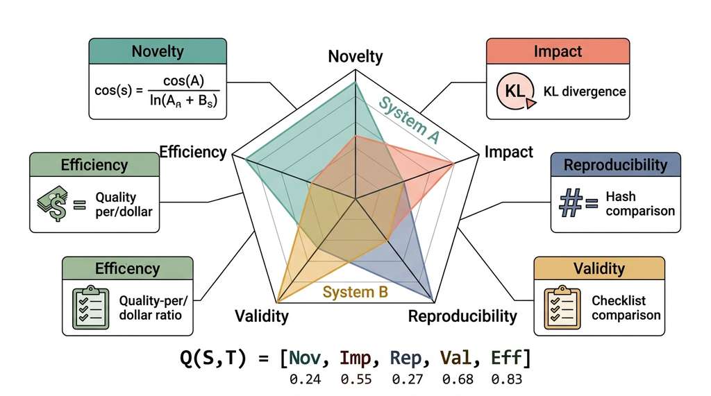
Five axes together capture the principal dimensions of discovery quality, as illustrated in Figure 56.1. Each axis is independent: a system can score high on one and low on another. These axes typically mirror the criteria that peer reviewers at top scientific journals apply, recast for automated and semi-automated measurement.
2.1 Novelty: Is It New?
Novelty measures the degree to which a discovery output differs from existing knowledge. A hypothesis that restates a well-known result has zero novelty; a hypothesis that proposes a previously unconsidered mechanism has high novelty. We formalize novelty using information-theoretic distance (a family of measures that quantify how different two representations are in terms of their information content).
Novelty scoring quantifies how different a candidate discovery is from everything already known. The score ranges from 0 (identical to prior work) to 1 (completely unprecedented). Without a formal novelty measure, a discovery system can game evaluations by rephrasing known results, producing outputs that look productive but add nothing to the knowledge frontier. The scorer encodes both the candidate and every item in the existing knowledge base as vectors in a shared embedding space, then computes the cosine distance to the nearest neighbor. A large minimum distance means the candidate occupies a region of concept space that no prior work has reached. Use embedding-based novelty when you have a large, well-indexed knowledge corpus and need fast, automated scoring; switch to expert panel review when the domain is too narrow for general-purpose embeddings to capture meaningful distinctions.
Let \(\mathcal{K}\) denote the corpus of existing knowledge (papers, databases, known results) and let \(d\) denote a candidate discovery. We define novelty as the minimum semantic distance between \(d\) and any element of \(\mathcal{K}\):
$$ \text{Novelty}(d) = \min_{k \in \mathcal{K}} \; \text{dist}(d, k) $$In practice, we embed both \(d\) and elements of \(\mathcal{K}\) into a shared vector space using a scientific language model and compute cosine distance (where cosine distance between two vectors is 1 minus the cosine of the angle between them, ranging from 0 for identical directions to 1 for orthogonal ones). A discovery is novel when it lies far from every known result in embedding space.
import numpy as np
from dataclasses import dataclass
from typing import List, Optional


@dataclass
class DiscoveryOutput:
    """A single output from a discovery system."""
    hypothesis: str
    evidence: List[str]
    methodology: str
    predicted_effect_size: Optional[float] = None
    compute_cost_seconds: float = 0.0
    token_cost: int = 0


def compute_novelty(
    discovery_embedding: np.ndarray,
    knowledge_embeddings: np.ndarray,
) -> float:
    """Compute novelty as max cosine distance to nearest known result.

    Args:
        discovery_embedding: (d,) vector for the candidate discovery
        knowledge_embeddings: (n, d) matrix of known results

    Returns:
        Novelty score in [0, 1] where 1 is maximally novel
    """
    # Normalize to unit vectors
    d_norm = discovery_embedding / (np.linalg.norm(discovery_embedding) + 1e-10)
    k_norms = knowledge_embeddings / (
        np.linalg.norm(knowledge_embeddings, axis=1, keepdims=True) + 1e-10
    )

    # Cosine similarity with every known result
    similarities = k_norms @ d_norm  # shape (n,)

    # Novelty = 1 - max_similarity (farther from known = more novel)
    max_similarity = np.max(similarities)
    return float(1.0 - max_similarity)
Common Misconception
A frequent mistake is treating novelty as a proxy for discovery quality: "if the system produces outputs far from existing knowledge, it must be doing well." In reality, random nonsense is also far from existing knowledge. High novelty without validity is noise, not discovery. Always evaluate novelty alongside the other four axes; a novelty score is meaningful only when the candidate has also passed validity and reproducibility checks.
A subtlety: novelty computed over a static knowledge corpus becomes stale as new papers appear. The Discovery Workbench addresses this by periodically re-indexing the knowledge base (see Chapter 37) and recomputing novelty scores against the updated corpus.
2.2 Impact: Does It Matter?
Novelty without impact is trivia. A discovery is impactful when it changes what scientists believe, what engineers build, or what clinicians prescribe. Impact is inherently forward-looking and difficult to measure at the time of discovery. We approximate it using two proxies.
Predicted downstream utility: How many existing open problems would this discovery help resolve? We measure this by counting the number of known open questions (from a curated problem bank or from research agendas) whose solution would be advanced by the discovery.
Information gain: How much does this discovery reduce uncertainty about the world? We formalize this as the KL divergence between the posterior belief after incorporating the discovery and the prior belief before it:
$$ \text{Impact}_{\text{info}}(d) = D_{\text{KL}}\bigl(P(\theta \mid d) \;\|\; P(\theta)\bigr) = \int P(\theta \mid d) \log \frac{P(\theta \mid d)}{P(\theta)} \, d\theta $$where \(\theta\) represents the parameters of a scientific model. A discovery that shifts the posterior substantially relative to the prior carries high information gain.
Mental Model
Think of information gain like a weather forecast that changes your plans. If tomorrow's forecast says "sunny, 25 C" in a region where it is sunny 350 days a year, you learn almost nothing and your plans stay the same (low KL divergence: the posterior barely differs from the prior). But if the forecast says "rare ice storm arriving tonight" in that same region, your beliefs shift dramatically and you reorganize your entire day (high KL divergence). A high-impact discovery is the scientific equivalent of that ice storm forecast: it forces the community to update its model of how the world works by a large amount, precisely because the new evidence is surprising relative to what was previously believed.
Consider a discovery system that proposes a new binding mechanism for a kinase inhibitor. The predicted downstream utility is high if there are active clinical trials targeting that kinase family. The information gain is high if the proposed mechanism contradicts the prevailing model of kinase selectivity, because it forces a large update in scientific beliefs. A system that merely confirms the existing selectivity model for a well-studied kinase would score low on both impact proxies, even if the finding is technically correct.
2.3 Reproducibility: Can Others Verify It?
A discovery that cannot be reproduced is, for practical purposes, not a discovery. The replication crisis in psychology, biomedicine, and social science has made reproducibility a first-class evaluation criterion. For AI discovery systems, reproducibility has two layers.
Computational reproducibility: Given the same inputs, code, and random seeds, does the system produce the same output? This is a prerequisite that Chapter 47 addresses through experiment registries and provenance tracking.
Scientific reproducibility: If the proposed experiment is actually conducted, do the results match the prediction? This requires either wet-lab validation or simulation with independently coded models.
import hashlib
import json


def check_computational_reproducibility(
    system_fn,
    inputs: dict,
    expected_hash: str,
    n_runs: int = 3,
) -> dict:
    """Verify that a discovery system produces identical outputs across runs.

    Args:
        system_fn: callable that takes inputs and returns a JSON-serializable result
        inputs: the input configuration
        expected_hash: SHA-256 hash of the canonical output
        n_runs: number of independent runs to check

    Returns:
        Dict with reproducibility verdict and details
    """
    hashes = []
    for run_idx in range(n_runs):
        result = system_fn(**inputs)
        result_json = json.dumps(result, sort_keys=True, default=str)
        run_hash = hashlib.sha256(result_json.encode()).hexdigest()
        hashes.append(run_hash)

    all_match = len(set(hashes)) == 1
    matches_expected = all_match and hashes[0] == expected_hash

    return {
        "computationally_reproducible": all_match,
        "matches_gold_standard": matches_expected,
        "unique_hashes": list(set(hashes)),
        "n_runs": n_runs,
    }
Checkpoint
So far: novelty measures how different a candidate is from known work, impact measures how much it would change scientific beliefs or practice, and reproducibility measures whether the result can be independently obtained again; the remaining two axes, validity and efficiency, address whether the finding is correct and what it costs to produce.
2.4 Validity: Is It Correct?
Reproducibility confirms that a result can be obtained again, but it says nothing about whether the result is right. Validity asks whether the discovery is actually true. A novel, impactful, reproducible finding that happens to be wrong is worse than useless because it consumes resources to refute. We decompose validity into three sub-dimensions.
Internal validity: Does the reasoning chain from evidence to conclusion hold? Are the statistical tests appropriate? Are the assumptions stated and justified? This can be partially automated by checking logical consistency and statistical methodology.
The three faces of validity
External validity: Does the finding generalize beyond the specific dataset or conditions? A pattern discovered in one cell line may not hold in others. External validity requires testing on held-out data or independent datasets.
Construct validity: Does the evaluation actually measure what it claims to measure? This meta-level concern, covered in depth in Section 56.3, is the most insidious because a flawed evaluation can make a broken system look excellent.
from enum import Enum


class ValidityLevel(Enum):
    """Levels of validation for a discovery output."""
    UNVALIDATED = 0        # No validation performed
    SELF_CONSISTENT = 1    # Passes internal logic checks
    COMPUTATIONALLY_VERIFIED = 2  # Verified by independent simulation
    EXPERIMENTALLY_CONFIRMED = 3  # Confirmed by wet-lab or field experiment
    INDEPENDENTLY_REPLICATED = 4  # Replicated by an independent group


def score_internal_validity(discovery: DiscoveryOutput) -> dict:
    """Check internal validity of a discovery output.

    Examines the reasoning chain for common statistical and logical errors.
    Returns a checklist of validity criteria with pass/fail status.
    """
    checks = {}

    # Check 1: evidence is provided
    checks["has_evidence"] = len(discovery.evidence) > 0

    # Check 2: methodology is specified
    checks["has_methodology"] = len(discovery.methodology.strip()) > 0

    # Check 3: effect size is quantified (not just "significant")
    checks["quantified_effect"] = discovery.predicted_effect_size is not None

    # Check 4: hypothesis is falsifiable (contains a testable prediction)
    falsifiable_markers = [
        "predict", "expect", "should", "will", "would increase",
        "would decrease", "correlate", "cause", "lead to",
    ]
    checks["falsifiable"] = any(
        marker in discovery.hypothesis.lower()
        for marker in falsifiable_markers
    )

    # Overall internal validity score
    checks["score"] = sum(checks.values()) / len(
        [k for k in checks if k != "score"]
    )

    return checks
2.5 Efficiency: At What Cost?
Two systems that produce equally novel, impactful, reproducible, and valid discoveries are not equally good if one costs a thousand times more. Efficiency measures the resource cost per unit of discovery quality. Resources include compute time, API token expenditure, wet-lab reagent cost, human expert time, and wall-clock latency.
We define a composite efficiency metric that normalizes discovery quality by cost:
$$ \text{Efficiency}(d) = \frac{Q(d)}{C(d)} $$where \(Q(d)\) is an aggregate quality score (a weighted combination of the other four axes) and \(C(d)\) is the total cost of producing discovery \(d\). This is analogous to the cost-performance Pareto frontier (the set of configurations where no axis can be improved without worsening another) described in Chapter 45.
@dataclass
class EvaluationCost:
    """Track all costs associated with producing a discovery."""
    compute_seconds: float = 0.0
    api_tokens: int = 0
    api_cost_usd: float = 0.0
    human_hours: float = 0.0
    lab_cost_usd: float = 0.0
    wall_clock_seconds: float = 0.0

    @property
    def total_cost_usd(self) -> float:
        """Estimate total cost in USD.

        Assumes $0.10/hr amortized compute and $150/hr for human experts.
        """
        compute_cost = self.compute_seconds / 3600 * 0.10
        human_cost = self.human_hours * 150
        return compute_cost + self.api_cost_usd + human_cost + self.lab_cost_usd


def compute_efficiency(
    quality_scores: dict,
    cost: EvaluationCost,
    quality_weights: Optional[dict] = None,
) -> float:
    """Compute cost-normalized discovery efficiency.

    Args:
        quality_scores: dict with keys novelty, impact, reproducibility, validity
        cost: EvaluationCost tracking all resource expenditures
        quality_weights: optional weighting; defaults to uniform

    Returns:
        Efficiency score (quality per dollar)
    """
    if quality_weights is None:
        quality_weights = {
            "novelty": 0.25,
            "impact": 0.25,
            "reproducibility": 0.25,
            "validity": 0.25,
        }

    aggregate_quality = sum(
        quality_weights.get(k, 0) * quality_scores.get(k, 0)
        for k in quality_weights
    )

    total_cost = max(cost.total_cost_usd, 0.01)  # avoid division by zero
    return aggregate_quality / total_cost
3. The Discovery Quality Vector
Combining all five axes, we define the discovery quality vector for a system \(S\) evaluated on a set of tasks \(\mathcal{T}\):
$$ \mathbf{Q}(S, \mathcal{T}) = \left[\overline{\text{Nov}}, \; \overline{\text{Imp}}, \; \overline{\text{Rep}}, \; \overline{\text{Val}}, \; \overline{\text{Eff}}\right] $$where each overbar denotes the mean score for that axis across all tasks in \(\mathcal{T}\). Reporting the full vector, rather than a single aggregate, lets practitioners identify the specific failure mode: a system that scores \([0.9, 0.8, 0.3, 0.7, 0.6]\) has a reproducibility problem that would be invisible in a weighted average. Figure 56.1.1 illustrates Five-axis Discovery Quality Vector.
@dataclass
class DiscoveryQualityVector:
    """The five-axis quality assessment for a discovery system."""
    novelty: float      # [0, 1]
    impact: float       # [0, 1]
    reproducibility: float  # [0, 1]
    validity: float     # [0, 1]
    efficiency: float   # [0, inf), but typically normalized to [0, 1]

    def to_array(self) -> np.ndarray:
        return np.array([
            self.novelty, self.impact,
            self.reproducibility, self.validity,
            self.efficiency,
        ])

    def weighted_aggregate(self, weights: Optional[np.ndarray] = None) -> float:
        """Compute weighted aggregate score. Use with caution."""
        if weights is None:
            weights = np.ones(5) / 5
        return float(weights @ self.to_array())

    def radar_plot_data(self) -> dict:
        """Return data formatted for radar/spider plot visualization."""
        labels = ["Novelty", "Impact", "Reproducibility", "Validity", "Efficiency"]
        values = self.to_array().tolist()
        return {"labels": labels, "values": values}


def evaluate_system(
    system_fn,
    tasks: list,
    knowledge_embeddings: np.ndarray,
    embedding_fn,
) -> DiscoveryQualityVector:
    """Run a discovery system on a task bank and compute the quality vector.

    This is the top-level evaluation function that orchestrates
    all five axis scorers.
    """
    novelty_scores = []
    validity_scores = []
    costs = []

    for task in tasks:
        # Run the system
        output = system_fn(task)
        cost = EvaluationCost(
            compute_seconds=output.compute_cost_seconds,
            api_tokens=output.token_cost,
        )
        costs.append(cost)

        # Score novelty
        emb = embedding_fn(output.hypothesis)
        nov = compute_novelty(emb, knowledge_embeddings)
        novelty_scores.append(nov)

        # Score internal validity
        val_result = score_internal_validity(output)
        validity_scores.append(val_result["score"])

    return DiscoveryQualityVector(
        novelty=float(np.mean(novelty_scores)),
        impact=0.0,  # requires human or LLM-judge scoring
        reproducibility=0.0,  # requires multi-run checking
        validity=float(np.mean(validity_scores)),
        efficiency=float(np.mean([
            1.0 / max(c.total_cost_usd, 0.01) for c in costs
        ])),
    )
evaluate_system function orchestrates scoring across all five axes. Impact and reproducibility require additional infrastructure (human judges and multi-run execution) that we build in Section 56.4.The hand-rolled evaluation code above handles scoring, but tracking results across system versions, comparing runs, and visualizing trends is a solved problem. MLflow's evaluation API handles all of this in roughly 10 lines:
import mlflow

with mlflow.start_run(run_name="discovery-system-v2.1"):
    mlflow.log_param("model", "claude-opus-4-20250514")
    mlflow.log_param("task_bank_version", "2024-Q4")

    # Log the full quality vector
    qv = evaluate_system(system_fn, tasks, knowledge_embs, embed_fn)
    mlflow.log_metric("novelty", qv.novelty)
    mlflow.log_metric("impact", qv.impact)
    mlflow.log_metric("reproducibility", qv.reproducibility)
    mlflow.log_metric("validity", qv.validity)
    mlflow.log_metric("efficiency", qv.efficiency)
    mlflow.log_metric("aggregate", qv.weighted_aggregate())
Six lines of logging replace an entire results database. MLflow provides versioned run comparison, metric visualization, and artifact storage. This reduces roughly 200 lines of custom tracking code to the snippet above.
4. Rubric Design for Human Evaluation
The quality vector and its automated scorers handle axes like novelty and reproducibility reasonably well, but impact and validity often require human judgment. The challenge is making that judgment consistent across raters. We achieve this through calibrated rubrics (structured scoring guides that pair each quality level with a concrete anchor example so that independent raters converge on the same score).
Table 56.1 shows a rubric for the impact axis. Each level has a verbal description and a concrete anchor example that raters study during calibration sessions before they begin scoring.
| Score | Level | Description | Anchor Example |
|---|---|---|---|
| 0 | No impact | Restates known results with no new insight | "Aspirin reduces inflammation" (known since 1897) |
| 1 | Incremental | Minor extension of existing work | Optimizing a known catalyst by 5% on a standard benchmark |
| 2 | Moderate | Solves a recognized open problem or enables a new method | A new featurization that improves molecular property prediction across datasets |
| 3 | High | Opens a new research direction or changes practice in a field | AlphaFold demonstrating that protein structure prediction is solvable with deep learning |
| 4 | Transformative | Fundamentally changes scientific understanding or creates a new field | CRISPR-Cas9 enabling programmable genome editing |
Section 56.3 develops the statistical machinery for ensuring raters apply these rubrics consistently (Cohen's kappa, a statistic measuring inter-rater agreement adjusted for chance, Krippendorff's alpha, its generalization to multiple raters and variable scales, and power analysis), and Section 56.4 integrates rubric-based human evaluation into the full evaluation suite.
A research team deploys a hypothesis generation agent (built using the architecture from Chapter 39) to propose mechanisms for antibiotic resistance in Klebsiella pneumoniae. Over one week, the agent produces 47 hypotheses. The evaluation team computes the quality vector:
- Novelty (0.72): 34 of 47 hypotheses have no close match in the PubMed corpus (cosine distance > 0.3 from all indexed abstracts).
- Impact (0.45): Two human experts rate each hypothesis using the Table 56.1 rubric. Most are scored as "incremental" (level 1), with three reaching "moderate" (level 2).
- Reproducibility (0.98): Rerunning the agent with the same seed produces 46 of 47 identical hypotheses; one varies due to a non-deterministic API call.
- Validity (0.61): Internal logic checks pass for 29 hypotheses. The remaining 18 cite retracted papers, assume conditions inconsistent with the organism, or propose untestable mechanisms.
- Efficiency (0.83): Total cost is \$12.40 in API calls and 3.2 hours of wall-clock time, producing roughly 2.3 valid novel hypotheses per dollar.
The quality vector \([0.72, 0.45, 0.98, 0.61, 0.83]\) reveals that the system is productively novel and computationally reliable, but its scientific validity needs improvement. The team traces the validity failures to the knowledge retrieval component and iterates on the retrieval-augmented generation (RAG) pipeline (see Chapter 37).
5. From Axes to Benchmarks
With the five axes defined and both automated scorers and human rubrics in hand, we have the vocabulary for discovery quality but not yet a shared test suite for cross-group comparison. A benchmark fills that gap: a standardized task set, gold-standard answers where available, and a scoring protocol that makes results comparable. The next section surveys the benchmarks the community has built for scientific discovery evaluation, examines what each measures, and identifies where gaps remain.
Research Frontier
In 2023, Boiko et al. introduced Coscientist (Nature, 2023), an LLM-driven autonomous agent that designs, plans, and executes real chemistry experiments by integrating web search, code execution, and robotic lab control. Coscientist demonstrates that discovery evaluation can no longer remain purely computational: the system's outputs are physical experimental results (e.g., successful palladium-catalyzed cross-coupling reactions), forcing evaluators to score validity and reproducibility against wet-lab ground truth rather than text-only proxies. Subsequent work on ScienceAgentBench (Hu et al., 2025) has begun formalizing multi-axis evaluation protocols for such end-to-end agent systems, but standardized benchmarks that cover all five axes described in this section remain an open problem.
Try It: Build a Novelty Scorer for ArXiv Abstracts
This mini-project builds a working novelty scorer using only a laptop and standard Python libraries. You will embed a small corpus of paper abstracts and score a new abstract against it.
Step 1. Install dependencies: pip install numpy scikit-learn requests.
Step 2. Use the ArXiv API to fetch 200 recent abstracts from a single
category (e.g., cs.AI). Parse the Atom XML response and extract the
<summary> field from each entry.
Step 3. Vectorize all 200 abstracts using
sklearn.feature_extraction.text.TfidfVectorizer with default settings. This
produces a sparse term frequency-inverse document frequency (TF-IDF) matrix serving as your knowledge corpus embeddings.
Step 4. Write your own abstract (or pick one from a different subfield, e.g.,
q-bio.BM) and transform it with the same vectorizer. Compute cosine similarity
against every corpus vector using sklearn.metrics.pairwise.cosine_similarity,
then compute novelty as 1 - max(similarities).
Step 5. Experiment with the boundary: try scoring an abstract you know is closely related to corpus papers (expect novelty near 0.2) and one from a distant field (expect novelty near 0.8). Plot a histogram of novelty scores for 20 test abstracts to see the distribution. Reflect on when TF-IDF novelty agrees or disagrees with your own judgment, and consider what a learned embedding model (e.g., Sentence-BERT) would capture that TF-IDF misses.
Exercise 56.1.1
A discovery system produces three hypotheses with novelty scores of 0.85, 0.12, and 0.60, and corresponding validity scores of 0.30, 0.95, and 0.70. A reviewer proposes ranking them by the product novelty × validity. Compute the product for each hypothesis, rank them, and then argue whether this ranking is appropriate. What failure mode does the product metric hide compared to reporting the full quality vector?
Hint
The products are 0.255, 0.114, and 0.420. Hypothesis C wins, but notice that hypothesis A has the highest novelty yet the lowest validity. A product ranking buries this diagnostic signal. Consider: if the team's goal is to identify promising but risky leads for further validation, is the product ranking still the right choice?
Step-Through: Computing a Novelty Score
Trace through the compute_novelty function with a tiny example. Suppose the
candidate discovery embedding is \(d = [0.6, 0.8]\) and the knowledge base contains two
known results: \(k_1 = [1.0, 0.0]\) and \(k_2 = [0.5, 0.5]\).
Step 1: Normalize. \(\|d\| = \sqrt{0.36 + 0.64} = 1.0\), so \(\hat{d} = [0.6, 0.8]\). \(\|k_1\| = 1.0\), so \(\hat{k}_1 = [1.0, 0.0]\). \(\|k_2\| = \sqrt{0.5} \approx 0.707\), so \(\hat{k}_2 = [0.707, 0.707]\).
Step 2: Cosine similarities. \(\text{sim}(d, k_1) = 0.6 \times 1.0 + 0.8 \times 0.0 = 0.600\). \(\text{sim}(d, k_2) = 0.6 \times 0.707 + 0.8 \times 0.707 = 0.990\).
Step 3: Novelty. \(\text{max\_similarity} = 0.990\), so \(\text{Novelty} = 1 - 0.990 = 0.010\). The candidate is very close to \(k_2\) in direction, so it scores nearly zero novelty. If we changed \(d\) to \([0.0, 1.0]\) (perpendicular to \(k_1\), further from \(k_2\)), novelty would rise to \(1 - 0.707 = 0.293\).
Real-World Application: Materials Discovery at A-Lab
The A-Lab at Lawrence Berkeley National Laboratory uses an autonomous system that proposes novel inorganic materials, synthesizes them with robotic equipment, and characterizes the results, all without human intervention. The lab evaluates its outputs along axes closely matching the five defined here: novelty is measured against the Inorganic Crystal Structure Database (ICSD), validity is confirmed by X-ray diffraction matching predicted structures, and efficiency is tracked as successful syntheses per robot-hour. In its first 17 days of operation (reported in Nature, 2023), A-Lab attempted 58 targets and successfully synthesized 41, demonstrating that multi-axis quality vectors are not just theoretical constructs but operational tools guiding real autonomous laboratories.
The Discovery That Almost Wasn't
When Barry Marshall proposed in 1982 that stomach ulcers were caused by the bacterium Helicobacter pylori, the hypothesis scored extraordinarily high on novelty (no one believed bacteria could survive in stomach acid) and potentially transformative on impact, but essentially zero on validity by the standards of the time: no peer reviewer accepted the evidence. Frustrated, Marshall drank a Petri dish of the bacteria, developed gastritis, and cured himself with antibiotics. He eventually won the 2005 Nobel Prize. The episode illustrates a deep tension in discovery evaluation: a scoring system that gates on current-evidence validity would have filtered out one of the most important medical discoveries of the 20th century.
Lab: Sensitivity of Novelty Scores to Embedding Choice
Goal: Discover how much the choice of text embedding model changes novelty rankings, and whether cheap embeddings (TF-IDF) agree with learned ones (Sentence-BERT).
Tools needed: Python 3.10+, scikit-learn,
sentence-transformers (the all-MiniLM-L6-v2 model), and
matplotlib. No GPU required.
Procedure (25 min): (1) Fetch 100 abstracts from ArXiv category
cs.CL using the ArXiv API. (2) Select 10 test abstracts from a different
category (e.g., astro-ph) and 10 from the same category. (3) For each test
abstract, compute novelty using TF-IDF cosine distance and separately using
Sentence-BERT cosine distance against the 100-abstract corpus. (4) Produce a scatter
plot of TF-IDF novelty (x-axis) vs. Sentence-BERT novelty (y-axis), coloring
same-category and cross-category points differently.
What to vary: Try swapping the corpus category, changing corpus size (50 vs.
200), and using a domain-specific model like allenai/specter2 instead of
MiniLM.
What to observe: Do the two embedding methods agree on which abstracts are most novel? Where do they disagree, and why? Does corpus size affect the ranking stability more than embedding choice?