Prerequisites
This section requires the benchmark survey from Section 56.2 and familiarity with basic statistical hypothesis testing (p-values, confidence intervals, Type I and Type II error). Readers who want a deeper treatment of inter-rater reliability should consult Krippendorff (2004) in the chapter bibliography.
A benchmark that appears to measure discovery capability may actually measure something else entirely: memorization of training data, sensitivity to prompt formatting, or the ability to game a narrow scoring protocol. This section catalogs the threats that undermine evaluation validity, provides tools for detecting the most common one (data contamination), and builds the human evaluation infrastructure needed to measure the axes (novelty, impact) that automated benchmarks miss. We cover Cohen's kappa and Krippendorff's alpha for inter-rater agreement, and statistical power analysis for determining how many evaluation instances are enough.
1. Construct Validity: Measuring What You Think You Measure
Imagine a team that spends six months optimizing a discovery agent to top a public leaderboard, only to learn that their benchmark was measuring the agent's ability to recall memorized training examples, not its capacity for genuine scientific reasoning. Construct validity, the degree to which a benchmark actually measures the theoretical construct it claims to measure, is the difference between these two outcomes. A benchmark with low construct validity produces numbers that are precise, reproducible, and meaningless.
Construct validity matters because every downstream decision rests on benchmark scores reflecting the capability you care about. Those decisions include which system to deploy, which research direction to fund, and which architecture to scale. The verification mechanism has three steps: define the theoretical construct (e.g., "ability to generate novel, testable hypotheses"), design tasks that require that construct, then check whether scores correlate with independent indicators (expert judgment, downstream task success, real-world deployment outcomes). Apply construct validity analysis whenever you introduce a new benchmark or adopt someone else's. Skip it only when you measure a well-established construct with a validated instrument, such as standard classification accuracy on a curated test set.
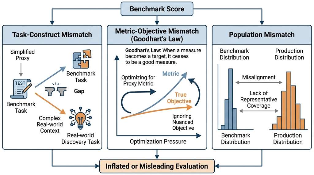
Three families of construct validity threats plague discovery evaluation. Figure 56.4 maps all three threat types to their corresponding detection and mitigation strategies. Figure 56.3.1 illustrates construct validity threat taxonomy for discovery benchmarks.
1.1 Task-Construct Mismatch
The benchmark tasks may not represent the real-world activity they claim to measure. ScienceAgentBench, for example, asks agents to reproduce published results from curated datasets. Real scientific discovery involves formulating questions, collecting data, navigating dead ends, and communicating findings to skeptical peers. Reproducing a known result is a necessary sub-skill, but treating reproduction performance as a proxy for discovery capability commits a mismatch error.
The general pattern: benchmark designers select tasks that are scorable (have verifiable answers) rather than tasks that are representative (reflect real-world usage). This creates a systematic bias toward measurable but narrow capabilities.
1.2 Metric-Objective Mismatch (Goodhart's Law)
Mental Model
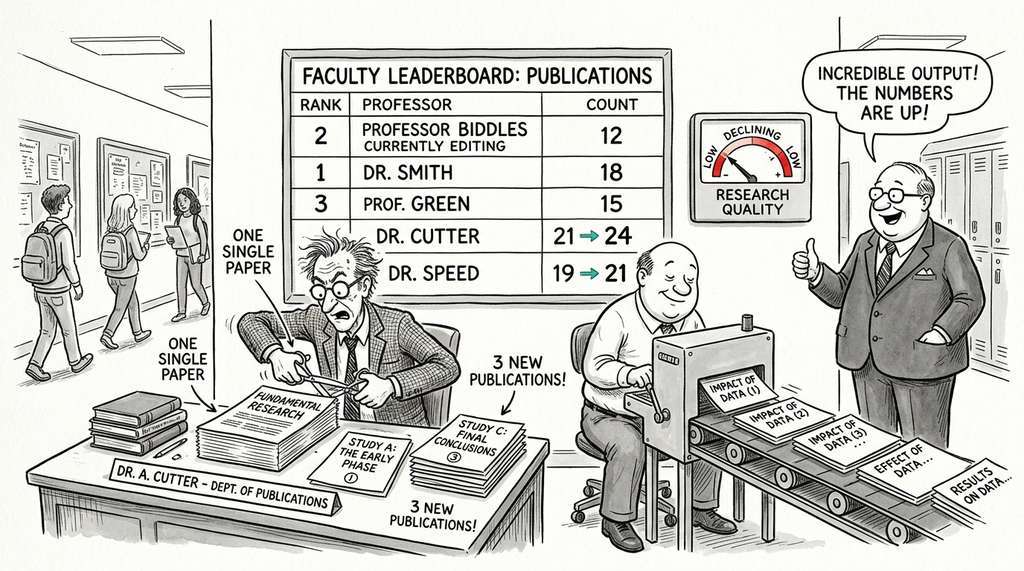
Think of Goodhart's Law like a university that ranks professors solely by publication count. At first, publication count correlates with research quality. But once professors know the metric, some start splitting one solid paper into three thin ones, or churning out incremental variations. The metric still rises, yet the thing it was supposed to track (research quality) stalls or declines. The same dynamic applies to discovery benchmarks: once a system is optimized to maximize the score, it finds shortcuts that inflate the number without improving the underlying capability the score was designed to reflect.
Goodhart's Law states: "When a measure becomes a target, it ceases to be a good measure." In the discovery context, optimizing a system for benchmark scores can degrade its real-world discovery performance. A system trained to maximize pass@1, where pass@1 is the probability that a single attempt produces a correct solution, on ScienceAgentBench may learn to produce conservative, template-following code that works on benchmark tasks but fails on novel problems that require creative approaches.
$$ \text{Goodhart gap} = \text{Perf}_{\text{real-world}}(S^*_{\text{real-world}}) - \text{Perf}_{\text{real-world}}(S^*_{\text{benchmark}}) $$
where \(S^*_{\text{benchmark}}\) is the system optimized for the benchmark and \(S^*_{\text{real-world}}\) is the system optimized directly for real-world performance. A positive Goodhart gap means the real-world-optimized system outperforms the benchmark-optimized system on actual deployment tasks, indicating that benchmark optimization has come at the expense of genuine capability.
1.3 Population Mismatch
The tasks in a benchmark may not represent the distribution of tasks a system will face in production. If a benchmark overrepresents computational chemistry and underrepresents genomics, a system that excels on the benchmark may fail on the genomics tasks that dominate a user's actual workload. This is the evaluation analog of domain shift in machine learning.
Each individual benchmark has blind spots. The only defense against construct validity threats is to evaluate on a portfolio of benchmarks that collectively cover the task distribution, scoring protocols, and capability dimensions that matter for your deployment context. The evaluation suite we build in Section 56.4 implements this portfolio approach, combining automated benchmarks with human evaluation to triangulate from multiple angles.
2. Data Contamination
Data contamination occurs when benchmark questions or answers appear in a model's training data, inflating scores through memorization rather than genuine reasoning. This is the most acute validity threat for large language model (LLM)-based discovery systems because web-scale training corpora inevitably overlap with published benchmarks.
2.1 Contamination Detection Methods
If contamination goes undetected, every score a team reports, every architecture decision it justifies, and every funding argument it builds on those scores rests on memorization masquerading as reasoning. The methods below exist because a single unaudited benchmark can silently invalidate months of engineering work.
Three methods detect contamination, each with different strengths.
N-gram overlap: Check whether benchmark questions appear verbatim (or near-verbatim) in known training corpora. This catches direct leakage but misses paraphrased versions.
Membership inference: Present the model with a benchmark question and measure its perplexity, where perplexity is a measure of how "surprised" the model is by the text (lower perplexity means higher familiarity). If the model is far more confident on benchmark questions than on similar but unseen questions, this suggests memorization (Oren et al., 2024).
Order sensitivity: Shuffle the answer choices in a multiple-choice question. If the model's accuracy depends on the original ordering (e.g., the correct answer was always option C in the training data), this indicates memorization rather than reasoning. In short: if shuffling the answers changes the score, the model remembers the test, not the subject.
import numpy as np
from typing import List, Tuple


def detect_contamination_by_order_sensitivity(
    model_fn,
    question: str,
    choices: List[str],
    correct_idx: int,
    n_permutations: int = 24,
    seed: int = 42,
) -> dict:
    """Detect memorization via answer-order sensitivity.

    If a model has memorized the question-answer pair, its accuracy
    will depend on whether the choices appear in their original order.
    A genuinely reasoning model should be order-invariant.

    Args:
        model_fn: callable(question, choices) -> predicted_index
        question: the question text
        choices: list of answer choice strings
        correct_idx: index of the correct answer in the original order
        n_permutations: number of random orderings to test
        seed: random seed for reproducibility

    Returns:
        Dict with contamination verdict and statistics
    """
    rng = np.random.default_rng(seed)
    n_choices = len(choices)

    original_correct = 0
    permuted_correct = 0
    original_trials = 0
    permuted_trials = 0

    for trial in range(n_permutations):
        perm = rng.permutation(n_choices)
        shuffled_choices = [choices[i] for i in perm]
        new_correct_idx = int(np.where(perm == correct_idx)[0][0])

        predicted = model_fn(question, shuffled_choices)
        is_correct = predicted == new_correct_idx

        # Check if this permutation is the original ordering
        is_original_order = list(perm) == list(range(n_choices))
        if is_original_order:
            original_correct += int(is_correct)
            original_trials += 1
        else:
            permuted_correct += int(is_correct)
            permuted_trials += 1

    original_accuracy = original_correct / max(original_trials, 1)
    permuted_accuracy = permuted_correct / max(permuted_trials, 1)

    # Large gap suggests memorization
    accuracy_gap = original_accuracy - permuted_accuracy

    return {
        "original_order_accuracy": original_accuracy,
        "permuted_order_accuracy": permuted_accuracy,
        "accuracy_gap": accuracy_gap,
        "likely_contaminated": accuracy_gap > 0.3,
        "n_permutations": n_permutations,
    }


def detect_contamination_by_perplexity(
    perplexity_fn,
    benchmark_questions: List[str],
    control_questions: List[str],
) -> dict:
    """Detect contamination via perplexity comparison.

    If the model has seen benchmark questions during training,
    it will assign them lower perplexity than similar but unseen
    control questions.

    Args:
        perplexity_fn: callable(text) -> float (perplexity score)
        benchmark_questions: questions from the benchmark being tested
        control_questions: similar questions NOT in any public benchmark

    Returns:
        Dict with contamination statistics
    """
    bench_perp = [perplexity_fn(q) for q in benchmark_questions]
    control_perp = [perplexity_fn(q) for q in control_questions]

    mean_bench = np.mean(bench_perp)
    mean_control = np.mean(control_perp)
    perplexity_ratio = mean_bench / (mean_control + 1e-10)

    # Statistical test: are benchmark perplexities significantly lower?
    from scipy import stats
    t_stat, p_value = stats.ttest_ind(bench_perp, control_perp, alternative="less")

    return {
        "mean_benchmark_perplexity": float(mean_bench),
        "mean_control_perplexity": float(mean_control),
        "perplexity_ratio": float(perplexity_ratio),
        "t_statistic": float(t_stat),
        "p_value": float(p_value),
        "likely_contaminated": p_value < 0.01 and perplexity_ratio < 0.8,
    }
Checkpoint
So far: three contamination detection methods target different evidence channels: n-gram overlap catches verbatim leakage, membership inference (perplexity comparison) catches familiarity with question text, and order sensitivity catches memorization of answer positions.
2.2 Mitigation Strategies
No single mitigation eliminates contamination, but several strategies reduce its impact:
- Dynamic benchmarks: SWE-bench Live continuously sources new issues that postdate model training cutoffs. This eliminates contamination at the cost of reduced curation quality. (As of 2025, several benchmarks have adopted this rolling-window model, including LiveCodeBench for code generation and LiveBench for general reasoning, establishing dynamic evaluation as a standard practice rather than an exception.)
- Private test sets: Keep a portion of the benchmark private, releasing only the development set. This is standard practice in shared tasks (e.g., SemEval) but requires a trusted evaluation server.
- Procedural generation: Generate tasks algorithmically so that each evaluation uses fresh instances. FrontierMath does this for mathematical problems.
- Contamination-adjusted scoring: Run contamination detection on each task and report separate scores for clean and potentially contaminated subsets.
Before publishing evaluation results for a new Discovery Workbench agent, the team runs a contamination audit on Graduate-Level Google-Proof Q&A (GPQA) Diamond. They apply the order-sensitivity test to all 198 questions. Results: 23 questions (11.6%) show an accuracy gap greater than 0.3 between original and permuted orderings, suggesting potential memorization. The team reports two accuracy numbers: 78.3% overall and 74.9% on the 175 "clean" questions. The 3.4 percentage point gap is within the range observed by Zhang et al. (2024), confirming that contamination inflates scores but does not account for all of the model's performance. This dual-reporting protocol becomes standard practice for all benchmark evaluations in the Discovery Workbench continuous integration (CI) pipeline.
3. Human Evaluation Protocols
Automated benchmarks cover validity and efficiency, but novelty and impact require human judgment. Reliable human evaluation rests on three pillars: annotator selection and training, statistical agreement measures, and power analysis for determining adequate sample sizes.
3.1 Annotator Selection and Training
For discovery evaluation, annotators must be domain experts: they need enough background to judge whether a hypothesis is genuinely novel (not just unfamiliar to them) and whether it addresses an important open problem (not just an interesting one). We recommend a minimum of three annotators per task, drawn from the relevant scientific domain, each with at least a graduate degree and active research experience.
Before scoring begins, annotators complete a calibration session: they independently score 10 pre-scored examples using the rubric from Section 56.1 (Table 56.1), then discuss disagreements in a group session. The calibration session often takes around 2 hours, depending on rubric complexity and domain familiarity, and tends to resolve most systematic differences in rubric interpretation.
3.2 Cohen's Kappa: Agreement Between Two Raters
Cohen's kappa (\(\kappa\)) measures the agreement between two raters beyond what would be expected by chance. Unlike raw percent agreement, kappa corrects for the possibility that raters agree on some items purely by coincidence. For two raters scoring \(n\) items into \(k\) categories, kappa is defined as:
$$ \kappa = \frac{p_o - p_e}{1 - p_e} $$where \(p_o\) is the observed proportion of agreement and \(p_e\) is the expected proportion of agreement under the assumption that raters assign categories independently according to their marginal distributions (the overall fraction of items each rater assigns to each category, ignoring which specific items received which labels). Values range from \(-1\) (complete disagreement) through \(0\) (chance agreement) to \(1\) (perfect agreement). The standard interpretation: \(\kappa < 0.20\) is poor, \(0.21\)-\(0.40\) is fair, \(0.41\)-\(0.60\) is moderate, \(0.61\)-\(0.80\) is substantial, and \(0.81\)-\(1.00\) is near-perfect.
import numpy as np
from typing import List, Tuple


def cohens_kappa(
    rater_a: List[int],
    rater_b: List[int],
) -> Tuple[float, str]:
    """Compute Cohen's kappa for two raters.

    Args:
        rater_a: list of category assignments from rater A
        rater_b: list of category assignments from rater B

    Returns:
        (kappa_value, interpretation_label)
    """
    assert len(rater_a) == len(rater_b), "Raters must score the same items"
    n = len(rater_a)

    # All unique categories across both raters
    categories = sorted(set(rater_a) | set(rater_b))
    k = len(categories)
    cat_to_idx = {c: i for i, c in enumerate(categories)}

    # Build confusion matrix
    confusion = np.zeros((k, k), dtype=int)
    for a, b in zip(rater_a, rater_b):
        confusion[cat_to_idx[a], cat_to_idx[b]] += 1

    # Observed agreement
    p_o = np.trace(confusion) / n

    # Expected agreement (product of marginals)
    row_sums = confusion.sum(axis=1) / n  # rater A marginals
    col_sums = confusion.sum(axis=0) / n  # rater B marginals
    p_e = float(row_sums @ col_sums)

    # Kappa
    if p_e == 1.0:
        kappa = 1.0  # both raters use only one category
    else:
        kappa = (p_o - p_e) / (1.0 - p_e)

    # Interpretation (Landis & Koch, 1977)
    if kappa > 0.80:
        label = "near-perfect"
    elif kappa > 0.60:
        label = "substantial"
    elif kappa > 0.40:
        label = "moderate"
    elif kappa > 0.20:
        label = "fair"
    else:
        label = "poor"

    return float(kappa), label


# Example: two experts rating 20 hypotheses on a 5-point impact scale
expert_a = [2, 3, 1, 2, 4, 1, 3, 2, 2, 1, 3, 2, 1, 4, 3, 2, 1, 2, 3, 2]
expert_b = [2, 3, 1, 3, 4, 1, 2, 2, 2, 1, 3, 2, 1, 4, 3, 2, 2, 2, 3, 2]

kappa, label = cohens_kappa(expert_a, expert_b)
print(f"Cohen's kappa: {kappa:.3f} ({label})")
# Cohen's kappa: 0.816 (near-perfect)
3.3 Krippendorff's Alpha: Agreement Among Multiple Raters
Cohen's kappa works for exactly two raters. When three or more annotators score each item (which we recommend for discovery evaluation), Krippendorff's alpha (\(\alpha\)) is the appropriate statistic. Alpha handles any number of raters, tolerates missing data (not every rater needs to score every item), and works with nominal, ordinal, interval, and ratio scales.
$$ \alpha = 1 - \frac{D_o}{D_e} $$where \(D_o\) is the observed disagreement and \(D_e\) is the expected disagreement under the null hypothesis of no systematic agreement. For ordinal data (which our impact rubric produces), the difference function uses squared rank differences: \(\delta^2(c, k) = (c - k)^2\).
import numpy as np
from itertools import combinations


def krippendorff_alpha(
    ratings_matrix: np.ndarray,
    level: str = "ordinal",
) -> float:
    """Compute Krippendorff's alpha for multiple raters.

    Args:
        ratings_matrix: (n_raters, n_items) array where NaN = missing.
            Each row is one rater; each column is one item.
        level: measurement level - "nominal", "ordinal", "interval", "ratio"

    Returns:
        Alpha coefficient in [-1, 1]
    """
    n_raters, n_items = ratings_matrix.shape

    # Difference function based on measurement level
    def delta_sq(v1, v2):
        if level == "nominal":
            return 0.0 if v1 == v2 else 1.0
        elif level in ("ordinal", "interval"):
            return (v1 - v2) ** 2
        elif level == "ratio":
            return ((v1 - v2) / (v1 + v2 + 1e-10)) ** 2
        else:
            raise ValueError(f"Unknown level: {level}")

    # Observed disagreement: average pairwise disagreement within each item
    d_o_total = 0.0
    n_pairs_total = 0

    for item_idx in range(n_items):
        values = ratings_matrix[:, item_idx]
        valid = values[~np.isnan(values)]
        m = len(valid)
        if m < 2:
            continue
        for i, j in combinations(range(m), 2):
            d_o_total += delta_sq(valid[i], valid[j])
            n_pairs_total += 1

    if n_pairs_total == 0:
        return 0.0

    D_o = d_o_total / n_pairs_total

    # Expected disagreement: average pairwise disagreement across all values
    all_values = ratings_matrix[~np.isnan(ratings_matrix)]
    n_total = len(all_values)

    d_e_total = 0.0
    n_e_pairs = 0
    # For efficiency, sample if the full comparison is too large
    if n_total > 1000:
        rng = np.random.default_rng(42)
        sample = rng.choice(all_values, size=1000, replace=False)
    else:
        sample = all_values

    for i, j in combinations(range(len(sample)), 2):
        d_e_total += delta_sq(sample[i], sample[j])
        n_e_pairs += 1

    D_e = d_e_total / max(n_e_pairs, 1)

    if D_e == 0:
        return 1.0  # perfect agreement and all values identical

    return 1.0 - (D_o / D_e)


# Example: three raters scoring 15 hypotheses on a 0-4 impact scale
ratings = np.array([
    [2, 3, 1, 2, 4, 1, 3, 2, 2, 1, 3, 2, np.nan, 4, 3],  # rater 1
    [2, 3, 1, 3, 4, 1, 2, 2, 2, 1, 3, 2, 1, 4, 3],        # rater 2
    [2, 2, 1, 2, 3, 1, 3, 2, 2, 1, 3, np.nan, 1, 4, 3],   # rater 3
])

alpha = krippendorff_alpha(ratings, level="ordinal")
print(f"Krippendorff's alpha: {alpha:.3f}")
# Krippendorff's alpha: 0.843
Common Misconception
A common misconception is that high inter-rater agreement (high kappa or alpha) means the rubric is measuring the right thing. It does not. Agreement statistics measure reliability (whether raters produce consistent scores), not validity (whether those scores capture the construct you care about). Three raters can perfectly agree on a score that systematically misses the point: for example, they might reliably rate "novelty" based on surface unfamiliarity rather than genuine scientific originality. Always validate what the rubric measures (construct validity, Section 1 above) separately from how consistently raters apply it.
The implementations above are pedagogical. In production, use established library implementations that handle edge cases and have been validated:
from sklearn.metrics import cohen_kappa_score
from nltk.metrics.agreement import AnnotationTask

# Cohen's kappa in one line
kappa = cohen_kappa_score(expert_a, expert_b, weights="quadratic")

# Krippendorff's alpha via NLTK
task_data = []
for rater_idx, rater_scores in enumerate(ratings):
    for item_idx, score in enumerate(rater_scores):
        if not np.isnan(score):
            task_data.append((f"r{rater_idx}", f"i{item_idx}", int(score)))

task = AnnotationTask(data=task_data)
alpha = task.alpha()
The sklearn
implementation also supports weighted kappa (linear, quadratic) for ordinal scales,
which penalizes large disagreements more than small ones.
4. Power Analysis: How Many Evaluation Instances?
A common failure in evaluation design is using too few instances to detect a meaningful difference between systems. Power analysis, a statistical planning technique that determines the minimum sample size needed to detect an effect of a given magnitude with a specified probability, prevents this failure by setting sample requirements before data collection begins.
The key parameters are:
- Effect size (\(d\)): The minimum difference between systems that we care about detecting. For discovery evaluation, a 5 to 10 percentage point difference is often considered meaningful, though the threshold depends on the cost and risk profile of the deployment context.
- Significance level (\(\alpha\)): The probability of a false positive (concluding that systems differ when they do not). Standard: \(\alpha = 0.05\).
- Power (\(1 - \beta\)): The probability of correctly detecting a real difference. Standard: \(1 - \beta = 0.80\).
- Variance (\(\sigma^2\)): The variability in scores across tasks. Higher variance requires larger samples.
For comparing two systems on a continuous metric (e.g., mean quality score), the required sample size per system is:
$$ n = \frac{2\sigma^2(z_{\alpha/2} + z_\beta)^2}{d^2} $$where \(z_{\alpha/2}\) and \(z_\beta\) are the standard normal quantiles corresponding to the significance level and Type II error rate.
from scipy import stats
import numpy as np


def power_analysis(
    effect_size: float,
    std_dev: float,
    alpha: float = 0.05,
    power: float = 0.80,
    test: str = "two-sample",
) -> dict:
    """Compute required sample size for comparing two systems.

    Args:
        effect_size: minimum detectable difference (e.g., 0.05 for 5pp)
        std_dev: estimated standard deviation of scores
        alpha: significance level (Type I error rate)
        power: desired statistical power (1 - Type II error rate)
        test: "two-sample" for independent systems, "paired" for same tasks

    Returns:
        Dict with required sample size and analysis parameters
    """
    beta = 1.0 - power
    z_alpha = stats.norm.ppf(1 - alpha / 2)
    z_beta = stats.norm.ppf(power)

    if test == "two-sample":
        n_per_group = int(np.ceil(
            2 * (std_dev ** 2) * (z_alpha + z_beta) ** 2 / (effect_size ** 2)
        ))
    elif test == "paired":
        # Paired test: need variance of differences, typically ~sqrt(2) * std_dev
        diff_std = std_dev * np.sqrt(2) * 0.7  # rough correlation correction
        n_per_group = int(np.ceil(
            (diff_std ** 2) * (z_alpha + z_beta) ** 2 / (effect_size ** 2)
        ))
    else:
        raise ValueError(f"Unknown test type: {test}")

    return {
        "n_per_group": n_per_group,
        "total_n": n_per_group * 2 if test == "two-sample" else n_per_group,
        "effect_size": effect_size,
        "std_dev": std_dev,
        "alpha": alpha,
        "power": power,
        "test": test,
    }


# Example: how many tasks do we need to detect a 5% accuracy difference?
result = power_analysis(
    effect_size=0.05,   # 5 percentage points
    std_dev=0.20,       # typical for binary accuracy
    alpha=0.05,
    power=0.80,
    test="paired",      # same tasks, two systems
)
print(f"Required tasks: {result['total_n']}")
# Required tasks: 246

# What about detecting a 10% difference?
result_10 = power_analysis(effect_size=0.10, std_dev=0.20)
print(f"Required tasks for 10pp difference: {result_10['total_n']}")
# Required tasks for 10pp difference: 126
The power analysis above reveals an uncomfortable truth: detecting a 5 percentage point difference between discovery systems requires roughly 250 evaluation instances. Many published evaluations use fewer than 100 tasks, which means they can only reliably detect differences of 10 percentage points or more. Smaller improvements, which are typical of iterative system refinement, will appear as noise rather than signal. Before concluding that two systems perform "similarly" on a small benchmark, compute the minimum detectable effect size. You may find that the evaluation simply could not have detected the difference, even if one exists.
5. Confidence Intervals via Bootstrap
Knowing how many instances to evaluate is only half the problem; you also need to quantify how much uncertainty remains in the scores those instances produce. Point estimates (e.g., "System A achieves 72.3% accuracy") are incomplete without confidence intervals. Bootstrapping, a resampling technique that repeatedly draws samples with replacement from the observed data to approximate the sampling distribution, provides nonparametric (making no assumptions about the underlying distribution shape) confidence intervals that work for any metric, including complex scoring protocols like medal rates and weighted quality vectors.
import numpy as np
from typing import Callable, Tuple


def bootstrap_ci(
    scores: np.ndarray,
    metric_fn: Callable = np.mean,
    confidence: float = 0.95,
    n_bootstrap: int = 10_000,
    seed: int = 42,
) -> Tuple[float, float, float]:
    """Compute bootstrap confidence interval for any metric.

    Args:
        scores: array of per-task scores
        metric_fn: function that maps an array of scores to a scalar
        confidence: confidence level (e.g., 0.95 for 95% CI)
        n_bootstrap: number of bootstrap samples
        seed: random seed

    Returns:
        (point_estimate, ci_lower, ci_upper)
    """
    rng = np.random.default_rng(seed)
    n = len(scores)

    point_estimate = float(metric_fn(scores))

    # Generate bootstrap distribution
    bootstrap_estimates = np.zeros(n_bootstrap)
    for i in range(n_bootstrap):
        sample = rng.choice(scores, size=n, replace=True)
        bootstrap_estimates[i] = metric_fn(sample)

    # Percentile method for CI
    alpha = 1 - confidence
    ci_lower = float(np.percentile(bootstrap_estimates, 100 * alpha / 2))
    ci_upper = float(np.percentile(bootstrap_estimates, 100 * (1 - alpha / 2)))

    return point_estimate, ci_lower, ci_upper


def compare_systems_bootstrap(
    scores_a: np.ndarray,
    scores_b: np.ndarray,
    metric_fn: Callable = np.mean,
    n_bootstrap: int = 10_000,
    seed: int = 42,
) -> dict:
    """Compare two systems using paired bootstrap test.

    Both systems must be evaluated on the same tasks (paired design).

    Returns:
        Dict with estimates, CIs, and p-value for the difference
    """
    assert len(scores_a) == len(scores_b), "Paired comparison requires same tasks"
    rng = np.random.default_rng(seed)
    n = len(scores_a)

    diff_scores = scores_a - scores_b
    observed_diff = float(metric_fn(scores_a) - metric_fn(scores_b))

    # Bootstrap the difference
    bootstrap_diffs = np.zeros(n_bootstrap)
    for i in range(n_bootstrap):
        idx = rng.choice(n, size=n, replace=True)
        bootstrap_diffs[i] = metric_fn(scores_a[idx]) - metric_fn(scores_b[idx])

    ci_lower = float(np.percentile(bootstrap_diffs, 2.5))
    ci_upper = float(np.percentile(bootstrap_diffs, 97.5))

    # Two-sided p-value: fraction of bootstrap diffs that cross zero
    p_value = float(np.mean(bootstrap_diffs <= 0) if observed_diff > 0
                    else np.mean(bootstrap_diffs >= 0))
    p_value = min(2 * p_value, 1.0)  # two-sided

    return {
        "system_a_mean": float(metric_fn(scores_a)),
        "system_b_mean": float(metric_fn(scores_b)),
        "mean_difference": observed_diff,
        "ci_95": (ci_lower, ci_upper),
        "p_value": p_value,
        "significant_at_05": p_value < 0.05,
    }


# Example: comparing two Discovery Workbench versions
rng = np.random.default_rng(42)
system_v1 = rng.binomial(1, 0.65, size=200).astype(float)  # 65% accuracy
system_v2 = rng.binomial(1, 0.72, size=200).astype(float)  # 72% accuracy

result = compare_systems_bootstrap(system_v2, system_v1)
print(f"Difference: {result['mean_difference']:.3f} "
      f"(95% CI: [{result['ci_95'][0]:.3f}, {result['ci_95'][1]:.3f}])")
print(f"p = {result['p_value']:.4f}, significant: {result['significant_at_05']}")
6. LLM-as-Judge: Scaling Human-Like Evaluation
The bootstrap machinery above produces rigorous comparisons once scores exist, but expert annotation is costly and slow. Since human evaluation does not scale to hundreds of discovery outputs per experiment cycle, teams need a way to approximate expert judgment automatically while retaining statistical rigor. An increasingly common alternative uses a frontier LLM as a judge, calibrated against human ratings on a subset. The judge receives the discovery output, the rubric, and anchor examples, then produces a score.
The critical validation step: compute the agreement between the LLM judge and human experts (using kappa or alpha) on a held-out calibration set. If agreement is "substantial" (\(\kappa > 0.60\)), the LLM judge can be used to score the remaining instances, with periodic human spot-checks. (As of 2025, LLM-as-judge protocols have matured significantly; frameworks such as Zheng et al.'s MT-Bench and Chatbot Arena (2023) established pairwise comparison methods, and subsequent work by Kim et al. (2024) on Prometheus 2 demonstrated that open-weight judge models, when fine-tuned on rubric-grounded feedback data, can approach proprietary-model agreement levels, broadening access to scalable evaluation.)
A team calibrates an LLM judge for the impact rubric. They collect human ratings from three domain experts on 50 discovery outputs (the calibration set). They prompt the LLM with the rubric, anchor examples, and each discovery output, and collect the LLM's ratings. Computing Cohen's kappa between the LLM and each human rater yields \(\kappa = 0.68\), \(0.71\), and \(0.65\) (substantial agreement). For comparison, inter-human kappa on the same set is \(\kappa = 0.74\), \(0.69\), and \(0.72\). The LLM judge agrees with each human about as well as the humans agree with each other, so the team uses it to score the remaining 500 evaluation instances, spot-checking 10% with human raters to detect drift.
Research Frontier
Mirzadeh et al. (2024) introduced GSM-Symbolic, a procedurally generated variant of the Grade School Math 8K (GSM8K) math benchmark in which names, numbers, and surface details are randomized for each evaluation run. Models that scored above 80% on the original GSM8K dropped by up to 15 percentage points on symbolically equivalent variants, demonstrating that a substantial fraction of reported performance reflected memorization of specific problem templates rather than general reasoning. This "template perturbation" approach extends naturally to discovery benchmarks: by programmatically varying dataset names, variable labels, and numerical parameters in tasks like ScienceAgentBench, evaluators can separate genuine analytical capability from shallow pattern matching against memorized training examples. LiveBench (White et al., 2024) takes a complementary approach, sourcing fresh questions monthly from recent information so that every evaluation window is provably uncontaminated.
Try It: Build a Contamination and Significance Detector
Test whether a language model has memorized a public benchmark, then determine whether two models differ significantly, using only Python and standard libraries.
Step 1. Pick 20 multiple-choice questions from a public benchmark (e.g., Massive Multitask Language Understanding (MMLU) or ARC-Challenge). Record the original answer ordering for each question.
Step 2. For each question, generate five random permutations of the
answer choices. Query a model API (or use a local model via
transformers) on each permutation and record whether the model selects
the correct answer. Compute the accuracy gap between the original ordering and the
permuted orderings using the detect_contamination_by_order_sensitivity
pattern from Listing 56.11.
Step 3. Repeat Step 2 with a second model. You now have per-question accuracy arrays for two models on the "clean" (permuted) orderings.
Step 4. Use the compare_systems_bootstrap function from
Listing 56.15 to compute a 95% confidence interval for the accuracy difference
between the two models on the clean subset. Report whether the difference is
statistically significant at \(p < 0.05\).
Step 5. Run power_analysis from Listing 56.14 with your
observed standard deviation and a target effect size of 5 percentage points.
Compare the recommended sample size to the 20 questions you used. Reflect on
whether your evaluation was adequately powered and how many questions you would
need for a publication-quality result.
Exercise 56.3.1
A benchmark for hypothesis generation contains 80 questions. Two raters independently label each hypothesis as "novel" or "not novel." Rater A labels 52 as novel; Rater B labels 48 as novel; they agree on 60 out of 80 items. Compute Cohen's kappa by hand. Then determine: is this agreement level sufficient to trust the rubric for a publication-quality evaluation? If not, what concrete step should the team take before proceeding?
Hint
First compute \(p_o = 60/80\). For \(p_e\), you need the probability that both raters say "novel" by chance plus the probability that both say "not novel" by chance. Rater A says "novel" with probability \(52/80\) and Rater B with probability \(48/80\). Use \(p_e = P(A{=}\text{novel}) \cdot P(B{=}\text{novel}) + P(A{=}\text{not}) \cdot P(B{=}\text{not})\). A kappa below 0.67 signals the need for a calibration session before scoring the full dataset.
Step-Through: Order-Sensitivity Contamination Detection
Trace through the order-sensitivity test with a tiny example: one question with four answer choices [A, B, C, D] where the correct answer is B (index 1).
Trial 1: Permutation = [A, B, C, D] (original order). Correct answer
is at index 1. Model predicts index 1. Correct. This is the original ordering, so
original_correct = 1, original_trials = 1.
Trial 2: Permutation = [C, D, A, B]. Correct answer (B) is now at
index 3. Model predicts index 1 (where B used to be). Wrong.
permuted_correct = 0, permuted_trials = 1.
Trial 3: Permutation = [D, A, B, C]. Correct answer (B) is now at
index 2. Model predicts index 1 again. Wrong.
permuted_correct = 0, permuted_trials = 2.
Result: original_accuracy = 1/1 = 1.0,
permuted_accuracy = 0/2 = 0.0,
accuracy_gap = 1.0 - 0.0 = 1.0. Since 1.0 > 0.3, the verdict is
likely_contaminated = True. The model always picks the original position
of the correct answer regardless of shuffling, a clear sign of memorization.
Real-World Application: HELM Benchmark Suite
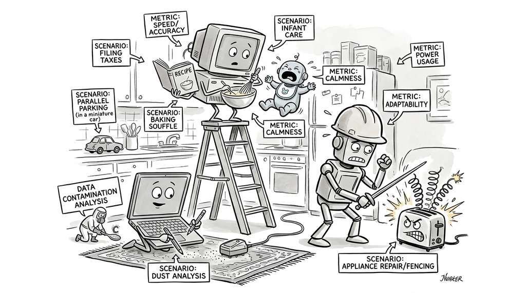
Stanford's Holistic Evaluation of Language Models (HELM) applies the portfolio approach from this section at industrial scale: it evaluates each model across dozens of scenarios, multiple metrics per scenario, and separate contamination analyses for every benchmark included. HELM reports contamination-adjusted scores alongside raw scores, letting practitioners see exactly how much leakage inflates each result. Organizations adopting HELM for internal model selection use its contamination flags to discount benchmarks where their fine-tuning data overlaps with test sets. (As of 2025, HELM has expanded into domain-specific variants, including HELM-Med for clinical evaluation and HELM-Lite for faster iteration, reflecting the broader trend toward modular, domain-adapted evaluation suites.)
The Benchmark That Graded Itself an A+
In 2023, researchers discovered that GPT-4's reported score on the US bar exam was inflated because bar exam prep materials (including questions nearly identical to the test) saturated the model's training corpus. When Martens et al. tested GPT-4 on a set of newly written bar-style questions with no online footprint, performance dropped by over 10 percentage points. The episode illustrates a recursive irony at the heart of contamination: the more famous and widely cited a benchmark becomes, the more likely it is to appear in future training data, which makes it less useful as a benchmark. Success breeds obsolescence.
Lab: Measuring Inter-Rater Agreement on LLM Outputs
Goal: Experience firsthand how rubric ambiguity affects agreement statistics, and calibrate your intuition for "good enough" kappa values.
Tools: Python with scikit-learn and numpy.
Optionally nltk for Krippendorff's alpha.
Procedure (20 minutes): (1) Prompt an LLM to generate 15 short
scientific hypotheses on a topic you know well. (2) Recruit two friends or colleagues
(or use two separate LLM sessions as simulated raters). Have each rater score all 15
hypotheses on a 1 to 5 novelty scale using a one-paragraph rubric you write yourself.
(3) Compute Cohen's kappa using sklearn.metrics.cohen_kappa_score with
weights="quadratic". (4) Hold a 5-minute calibration discussion where
raters compare their most divergent scores. (5) Re-score the 5 hypotheses with the
largest disagreements. Recompute kappa.
What to vary: Try a vague rubric ("rate novelty from 1 to 5") versus a detailed rubric with anchor examples for each level. Compare the kappa values.
What to observe: How much does kappa improve after calibration? How much does rubric specificity matter? Typical result: vague rubrics yield kappa around 0.3 to 0.5; detailed rubrics with anchors reach 0.6 to 0.8 even before calibration.