12.4 Building a Scientific MCP Server

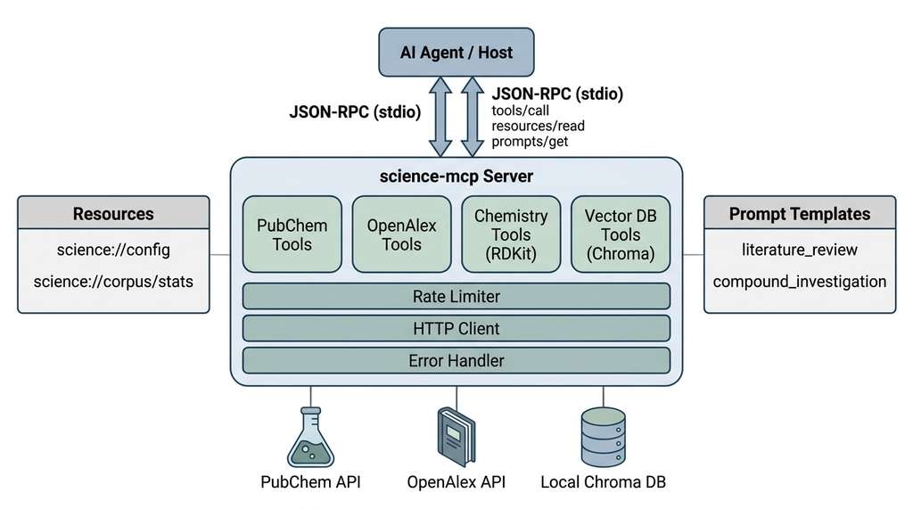
Figure 12.3 shows the layered architecture of the science-mcp server. An AI agent (or human client) communicates through the MCP protocol layer, which routes requests to the appropriate tool module. Each module wraps a distinct backend: PubChem for compound data, OpenAlex for literature, and the Chroma vector database for the lab's private corpus. Shared infrastructure (rate limiting, HTTP pooling, error handling) sits beneath all three, so adding a new backend means writing one module without touching the others.

1. Project Structure

Imagine typing a single question and watching an agent search PubChem for molecular data, query OpenAlex for related papers, and scan your lab's private notebook for prior experiments on the same compound. Building a server that orchestrates all three requires a project structure where adding the twentieth tool is nearly as straightforward as adding the second.

science-mcp/
├── pyproject.toml
├── README.md
├── src/
│   └── science_mcp/
│       ├── __init__.py
│       ├── server.py            # Entry point: creates Server, registers all tools
│       ├── config.py            # Configuration from environment variables
│       ├── utils/
│       │   ├── __init__.py
│       │   ├── rate_limiter.py  # Token-bucket rate limiter
│       │   ├── http_client.py   # Shared async HTTP client
│       │   └── errors.py        # Structured error responses
│       ├── tools/
│       │   ├── __init__.py
│       │   ├── pubchem.py       # PubChem compound search and lookup
│       │   ├── literature.py    # OpenAlex literature search
│       │   ├── chemistry.py     # RDKit molecular computation
│       │   └── vector_db.py     # Chroma vector database search
│       ├── resources/
│       │   ├── __init__.py
│       │   └── corpus.py        # Corpus metadata and configuration resources
│       └── prompts/
│           ├── __init__.py
│           └── workflows.py     # Scientific workflow prompt templates
├── tests/
│   ├── conftest.py
│   ├── test_pubchem.py
│   ├── test_literature.py
│   ├── test_chemistry.py
│   ├── test_vector_db.py
│   └── test_protocol.py
└── Dockerfile

2. Configuration Management

Scientific MCP servers need configuration for API endpoints, authentication tokens, database paths, and rate limits. Environment variables are the standard mechanism (as covered in Section 12.3), but a configuration module provides validation, defaults, and documentation.

"""Configuration for the science-mcp server."""
import os
from dataclasses import dataclass, field


@dataclass(frozen=True)
class Config:
    """Server configuration loaded from environment variables.

    All settings have sensible defaults for local development.
    Production deployments should set API keys and adjust rate limits.
    """
    # OpenAlex settings
    openalex_email: str = field(
        default_factory=lambda: os.environ.get("OPENALEX_EMAIL", "user@example.com")
    )
    openalex_rate_limit: float = field(
        default_factory=lambda: float(os.environ.get("OPENALEX_RATE_LIMIT", "10.0"))
    )

    # PubChem settings
    pubchem_rate_limit: float = field(
        default_factory=lambda: float(os.environ.get("PUBCHEM_RATE_LIMIT", "5.0"))
    )

    # Vector database settings
    chroma_persist_dir: str = field(
        default_factory=lambda: os.environ.get("CHROMA_PERSIST_DIR", "./chroma_data")
    )
    chroma_collection: str = field(
        default_factory=lambda: os.environ.get("CHROMA_COLLECTION", "scientific_papers")
    )
    embedding_model: str = field(
        default_factory=lambda: os.environ.get(
            "EMBEDDING_MODEL", "all-MiniLM-L6-v2"
        )
    )

    # Server settings
    server_name: str = "science-mcp"
    server_version: str = "1.0.0"
    max_concurrent_requests: int = field(
        default_factory=lambda: int(os.environ.get("MAX_CONCURRENT", "10"))
    )


def load_config() -> Config:
    """Load and validate server configuration."""
    config = Config()
    # Warn about defaults in production
    if config.openalex_email == "user@example.com":
        import warnings
        warnings.warn(
            "OPENALEX_EMAIL not set. Using default. "
            "Set it to join the OpenAlex polite pool for higher rate limits.",
            stacklevel=2,
        )
    return config

The default embedding model, all-MiniLM-L6-v2, is a solid lightweight choice (384 dimensions, fast inference). As of 2025, newer models such as nomic-embed-text-v1.5 and gte-large-en-v1.5 offer improved retrieval quality on scientific text at comparable inference cost; swap the EMBEDDING_MODEL environment variable to experiment.

3. The Vector Database Tool

With configuration in place, we can turn to the tools themselves; the PubChem and OpenAlex integrations follow the patterns from Section 12.2, so here we focus on the component those earlier tools lacked: a vector database for semantic search over local documents.

The server's third tool domain is a vector database for semantic search over local documents. PubChem and OpenAlex search public databases; the vector database searches your collection: lab papers, internal reports, experiment notes, proprietary datasets. These Retrieval Augmented Discovery patterns develop fully in Chapter 37.

Labs lose months of work when researchers unknowingly repeat experiments that a colleague already ran under a different name or notation. A search layer that understands meaning, not just keywords, is what prevents that costly duplication.

A vector database stores high-dimensional numerical vectors, where each vector represents the meaning of a piece of text, an image, or any data that an embedding model can encode. Traditional keyword search fails when the query and the relevant document use different words for the same concept. A search for "heart attack treatment" misses a paper titled "myocardial infarction therapy" because the words do not overlap, even though the meaning does. An embedding model converts both documents and queries into fixed-length vectors in the same high-dimensional space. The database then uses approximate nearest-neighbor algorithms (such as Hierarchical Navigable Small World (HNSW) graphs) to locate the stored vectors closest to the query vector, typically typically in milliseconds even over millions of documents. Use a vector database when your search needs are semantic (meaning-based) rather than exact-match; for structured lookups by known identifiers or precise field values, a traditional relational or document database remains the better choice.

We use Chroma, an open-source embedding database that stores documents as vectors and retrieves them by semantic similarity. When a user queries "CRISPR delivery mechanisms in neurons," Chroma encodes the query into a vector using the same embedding model that encoded the documents, then returns the documents whose vectors are closest in cosine distance. In short: the protocol turns three separate databases into one coherent scientific instrument that any agent can pick up and use.

The cosine similarity between two embedding vectors \(\mathbf{a}\) and \(\mathbf{b}\) is:

Values range from \(-1\) (opposite) to \(1\) (identical). For normalized embeddings (which most sentence transformers produce), this simplifies to a dot product. Chroma handles the indexing, storage, and nearest-neighbor search; we only need to wrap it as an MCP tool.

"""Vector database tools using Chroma for semantic search."""
import json
from mcp.server import Server
import chromadb
from chromadb.config import Settings

server = Server("vector-db-tools")

# Initialize Chroma client (persistent storage)
_chroma_client: chromadb.ClientAPI | None = None
_collection: chromadb.Collection | None = None


def get_collection(persist_dir: str, collection_name: str) -> chromadb.Collection:
    """Lazy-initialize the Chroma collection."""
    global _chroma_client, _collection
    if _collection is None:
        _chroma_client = chromadb.PersistentClient(
            path=persist_dir,
            settings=Settings(anonymized_telemetry=False),
        )
        _collection = _chroma_client.get_or_create_collection(
            name=collection_name,
            metadata={"hnsw:space": "cosine"},
        )
    return _collection


@server.tool()
async def search_corpus(
    query: str,
    max_results: int = 5,
    min_relevance: float = 0.3,
    metadata_filter: dict | None = None,
) -> str:
    """Search the local scientific corpus by semantic similarity.

    Finds documents in the local vector database whose content is
    semantically similar to the query. Useful for finding relevant
    papers, notes, or reports in the lab's private collection.

    Args:
        query: Natural language search query.
               Example: 'mechanisms of drug resistance in cancer cells'.
        max_results: Maximum documents to return (1-20, default 5).
        min_relevance: Minimum cosine similarity score (0.0 to 1.0).
                       Documents below this threshold are excluded.
        metadata_filter: Optional filter on document metadata.
                         Example: {"year": {"$gte": 2023}, "type": "paper"}.

    Returns:
        JSON with matching documents sorted by relevance. Each document
        includes: id, text (excerpt), metadata, and relevance_score.
    """
    collection = get_collection("./chroma_data", "scientific_papers")

    query_params = {
        "query_texts": [query],
        "n_results": min(max_results, 20),
    }
    if metadata_filter:
        query_params["where"] = metadata_filter

    results = collection.query(**query_params)

    documents = []
    for i in range(len(results["ids"][0])):
        # Chroma returns distances; convert to similarity for cosine
        distance = results["distances"][0][i] if results["distances"] else 0
        similarity = 1 - distance  # cosine distance to similarity

        if similarity < min_relevance:
            continue

        documents.append({
            "id": results["ids"][0][i],
            "text": results["documents"][0][i][:1000],  # Truncate for context window
            "metadata": results["metadatas"][0][i] if results["metadatas"] else {},
            "relevance_score": round(similarity, 4),
        })

    return json.dumps({
        "documents": documents,
        "count": len(documents),
        "query": query,
        "source": "local_corpus",
    }, indent=2)


@server.tool()
async def add_to_corpus(
    text: str,
    doc_id: str,
    metadata: dict | None = None,
) -> str:
    """Add a document to the local scientific corpus.

    Indexes a document for future semantic search. Use this to build
    a searchable collection of papers, notes, and experimental results.

    Args:
        text: The document text to index. Can be an abstract, full paper,
              or experiment note. Long documents should be chunked first.
        doc_id: Unique identifier for the document (e.g., 'doi:10.1234/example').
        metadata: Optional metadata dict. Recommended keys:
                  'title', 'authors', 'year', 'type' (paper/note/report),
                  'source' (pubmed/arxiv/internal).

    Returns:
        Confirmation with the document ID and metadata.
    """
    collection = get_collection("./chroma_data", "scientific_papers")

    collection.upsert(
        ids=[doc_id],
        documents=[text],
        metadatas=[metadata or {}],
    )

    return json.dumps({
        "status": "indexed",
        "doc_id": doc_id,
        "metadata": metadata or {},
        "text_length": len(text),
        "collection_size": collection.count(),
    }, indent=2)

The add_to_corpus docstring notes that "long documents should be chunked first," and in practice this step is essential. Embedding models have a fixed input window (typically 256 to 512 tokens for sentence transformers), so a 20-page paper fed in whole will be truncated, losing most of its content. Chunking splits a long document into overlapping segments (for example, 300-word passages with a 50-word overlap) so that each segment fits the model's window and gets its own vector. A query can then match the specific passage that discusses the relevant concept rather than competing against a single diluted vector for the entire paper. Chapter 37 on Retrieval Augmented Discovery covers chunking strategies in detail; for now, keep passages short enough to fit your embedding model's context window.

4. Resources: Server Metadata and Corpus Statistics

Beyond tools, our server exposes resources that provide context without requiring computation. Resources are ideal for metadata that the agent (or the human) might need to understand the server's capabilities and the state of the local corpus.

"""MCP resources for server metadata and corpus statistics."""
import json
from mcp.server import Server

server = Server("science-mcp")

@server.resource("science://config")
async def get_server_config() -> str:
    """Current server configuration and capability summary.

    Returns which APIs are configured, rate limits, and vector database status.
    Useful for the agent to understand what tools are available and any
    constraints on their use.
    """
    config = load_config()
    collection = get_collection(config.chroma_persist_dir, config.chroma_collection)

    return json.dumps({
        "server": {
            "name": config.server_name,
            "version": config.server_version,
        },
        "apis": {
            "pubchem": {
                "enabled": True,
                "rate_limit_per_second": config.pubchem_rate_limit,
            },
            "openalex": {
                "enabled": True,
                "rate_limit_per_second": config.openalex_rate_limit,
                "polite_pool": config.openalex_email != "user@example.com",
            },
        },
        "vector_database": {
            "backend": "chroma",
            "collection": config.chroma_collection,
            "document_count": collection.count(),
            "embedding_model": config.embedding_model,
        },
    }, indent=2)


@server.resource("science://corpus/stats")
async def get_corpus_stats() -> str:
    """Statistics about the local scientific corpus.

    Returns document count, metadata distribution, and storage usage.
    Helps the agent decide whether to search the local corpus or
    external databases for a given query.
    """
    config = load_config()
    collection = get_collection(config.chroma_persist_dir, config.chroma_collection)

    # Get metadata distribution
    all_metadata = collection.get(include=["metadatas"])
    total = len(all_metadata["ids"])

    type_counts = {}
    year_counts = {}
    for meta in (all_metadata["metadatas"] or []):
        doc_type = meta.get("type", "unknown")
        type_counts[doc_type] = type_counts.get(doc_type, 0) + 1
        year = meta.get("year")
        if year:
            year_counts[str(year)] = year_counts.get(str(year), 0) + 1

    return json.dumps({
        "total_documents": total,
        "by_type": type_counts,
        "by_year": dict(sorted(year_counts.items())),
        "collection_name": config.chroma_collection,
    }, indent=2)

5. Prompt Templates for Scientific Workflows

Resources give the agent a read-only window into the server's state, but they do not tell it how to combine tools into a coherent investigation; that guidance comes from prompt templates.

Prompt templates encode common scientific workflows as reusable, parameterized instructions. They guide the agent through multi-step processes that combine several tools in a specific order. Think of them as recipes: the agent supplies the ingredients (a compound name, a research question), and the prompt template supplies the procedure.

"""Scientific workflow prompt templates."""
from mcp.server import Server
from mcp.types import PromptMessage, TextContent

server = Server("science-mcp")

@server.prompt()
async def literature_review(
    topic: str,
    year_from: int = 2020,
    max_papers: int = 10,
) -> list[PromptMessage]:
    """Generate a structured literature review workflow.

    Args:
        topic: Research topic to review (e.g., 'AlphaFold protein structure prediction').
        year_from: Earliest publication year to include.
        max_papers: Maximum papers to retrieve.
    """
    return [
        PromptMessage(
            role="user",
            content=TextContent(
                type="text",
                text=(
                    f"Conduct a structured literature review on: {topic}\n\n"
                    f"Follow these steps:\n\n"
                    f"1. Use search_literature to find the {max_papers} most-cited "
                    f"papers on '{topic}' published since {year_from}.\n\n"
                    f"2. Use search_corpus to check if our local collection has "
                    f"related papers or notes on this topic.\n\n"
                    f"3. For each paper found, extract:\n"
                    f"   - Key contribution (one sentence)\n"
                    f"   - Methodology\n"
                    f"   - Main findings\n"
                    f"   - Limitations noted by the authors\n\n"
                    f"4. Identify research gaps: what questions remain open?\n\n"
                    f"5. Synthesize findings into a structured summary with sections:\n"
                    f"   - Background and motivation\n"
                    f"   - Methods landscape\n"
                    f"   - Key results across studies\n"
                    f"   - Open questions and future directions\n\n"
                    f"6. Use add_to_corpus to save the review summary for future reference."
                ),
            ),
        )
    ]


@server.prompt()
async def compound_investigation(smiles: str) -> list[PromptMessage]:
    """Generate a comprehensive compound investigation workflow.

    Args:
        smiles: SMILES notation of the compound to investigate.
    """
    return [
        PromptMessage(
            role="user",
            content=TextContent(
                type="text",
                text=(
                    f"Investigate the compound: {smiles}\n\n"
                    f"Follow these steps:\n\n"
                    f"1. Use compute_descriptors to calculate physicochemical "
                    f"properties and drug-likeness.\n\n"
                    f"2. Use search_pubchem with the SMILES to find the compound "
                    f"in PubChem and get its CID, name, and known activities.\n\n"
                    f"3. Use find_similar_compounds to identify structural analogs.\n\n"
                    f"4. Use search_literature with the compound name to find "
                    f"published studies.\n\n"
                    f"5. Use search_corpus to check for internal data on this "
                    f"compound or its analogs.\n\n"
                    f"6. Synthesize all findings into a compound profile:\n"
                    f"   - Identity (name, formula, structure)\n"
                    f"   - Physicochemical properties and drug-likeness\n"
                    f"   - Known biological activities\n"
                    f"   - Structural analogs and their activities\n"
                    f"   - Literature context\n"
                    f"   - Internal lab data (if any)\n"
                    f"   - Recommendation: pursue, deprioritize, or investigate further"
                ),
            ),
        )
    ]

6. The Complete Server Entry Point

The entry point ties everything together: it loads configuration, initializes shared infrastructure, registers all tools, resources, and prompts, and starts the stdio transport loop (where stdio, short for standard input/output, means the server reads JSON-RPC requests from its stdin stream and writes responses to stdout, letting the host launch it as a simple child process with no network configuration). Figure 12.4.1 illustrates science-mcp server architecture.

"""science-mcp: A unified MCP server for scientific discovery.

Combines PubChem compound search, OpenAlex literature search,
RDKit molecular computation, and Chroma vector database into
a single MCP server for scientific discovery workflows.
"""
import asyncio
import logging
from mcp.server import Server
from mcp.server.stdio import stdio_server

from science_mcp.config import load_config
from science_mcp.utils.http_client import SharedHTTPClient
from science_mcp.utils.rate_limiter import RateLimiter

# Configure logging
logging.basicConfig(
    level=logging.INFO,
    format="%(asctime)s [%(name)s] %(levelname)s: %(message)s",
)
logger = logging.getLogger("science-mcp")


def create_server() -> Server:
    """Create and configure the MCP server with all tools and resources."""
    config = load_config()
    server = Server(config.server_name)

    # Shared infrastructure
    http_client = SharedHTTPClient()
    pubchem_limiter = RateLimiter(rate=config.pubchem_rate_limit, burst=5)
    openalex_limiter = RateLimiter(rate=config.openalex_rate_limit, burst=10)

    # --- PubChem Tools ---
    @server.tool()
    async def search_pubchem(
        query: str, search_type: str = "name", max_results: int = 5
    ) -> str:
        """Search PubChem for chemical compounds by name, formula, or SMILES.

        Args:
            query: Search term (compound name, formula, or SMILES string).
            search_type: One of 'name', 'formula', or 'smiles'.
            max_results: Number of results (1-25, default 5).

        Returns:
            JSON with compounds array (cid, name, formula, weight, smiles).
        """
        await pubchem_limiter.acquire()
        client = await http_client.get()
        # ... full implementation from Section 12.2 ...

    @server.tool()
    async def get_compound_properties(cid: int) -> str:
        """Get detailed properties for a PubChem compound by CID.

        Args:
            cid: PubChem Compound ID (positive integer, e.g., 2244 for aspirin).

        Returns:
            JSON with compound properties including name, formula, weight,
            SMILES, InChI, and computed descriptors.
        """
        await pubchem_limiter.acquire()
        client = await http_client.get()
        # ... implementation ...

    # --- OpenAlex Tools ---
    @server.tool()
    async def search_literature(
        query: str,
        max_results: int = 10,
        sort_by: str = "relevance",
        year_from: int | None = None,
        year_to: int | None = None,
        open_access_only: bool = False,
    ) -> str:
        """Search scholarly literature using OpenAlex.

        Args:
            query: Search terms. Supports boolean operators ('AND', 'OR').
            max_results: Number of papers (1-50, default 10).
            sort_by: One of 'relevance', 'cited_by_count', 'publication_date'.
            year_from: Earliest publication year.
            year_to: Latest publication year.
            open_access_only: Return only open-access papers.

        Returns:
            JSON with papers array (title, authors, year, doi, abstract,
            cited_by_count, open_access_url) and total_count.
        """
        await openalex_limiter.acquire()
        client = await http_client.get()
        # ... full implementation from Section 12.2 ...

    # --- Chemistry Computation Tools ---
    @server.tool()
    async def compute_descriptors(smiles: str) -> str:
        """Compute physicochemical descriptors and drug-likeness for a molecule.

        Args:
            smiles: Molecule in SMILES notation (e.g., 'CCO' for ethanol).

        Returns:
            JSON with molecular descriptors (MW, LogP, HBD, HBA, TPSA,
            rotatable bonds) and Lipinski Rule of Five assessment.
        """
        # ... full implementation from Section 12.2 ...

    @server.tool()
    async def find_similar_compounds(
        smiles: str, threshold: float = 0.7, fingerprint: str = "morgan"
    ) -> str:
        """Find structurally similar compounds using molecular fingerprints.

        Args:
            smiles: Query molecule in SMILES notation.
            threshold: Minimum Tanimoto similarity (0.0-1.0, default 0.7).
            fingerprint: Algorithm ('morgan' or 'rdkit', default 'morgan').

        Returns:
            JSON with similar compounds sorted by decreasing similarity.
        """
        # ... full implementation from Section 12.2 ...

    # --- Vector Database Tools ---
    @server.tool()
    async def search_corpus(
        query: str, max_results: int = 5, min_relevance: float = 0.3
    ) -> str:
        """Search the local scientific corpus by semantic similarity.

        Args:
            query: Natural language query (e.g., 'CRISPR delivery in neurons').
            max_results: Maximum documents (1-20, default 5).
            min_relevance: Minimum cosine similarity (0.0-1.0, default 0.3).

        Returns:
            JSON with matching documents (id, text excerpt, metadata, score).
        """
        # ... full implementation from above ...

    @server.tool()
    async def add_to_corpus(
        text: str, doc_id: str, metadata: dict | None = None
    ) -> str:
        """Add a document to the local scientific corpus for future search.

        Args:
            text: Document text to index (abstract, paper, or note).
            doc_id: Unique identifier (e.g., 'doi:10.1234/example').
            metadata: Optional dict with 'title', 'authors', 'year', 'type'.

        Returns:
            Confirmation with document ID and updated corpus size.
        """
        # ... full implementation from above ...

    # --- Resources ---
    @server.resource("science://config")
    async def get_server_config() -> str:
        """Server configuration, API status, and rate limits."""
        # ... implementation from above ...

    @server.resource("science://corpus/stats")
    async def get_corpus_stats() -> str:
        """Corpus statistics: document count, type distribution, year range."""
        # ... implementation from above ...

    # --- Prompts ---
    @server.prompt()
    async def literature_review(
        topic: str, year_from: int = 2020, max_papers: int = 10
    ) -> list:
        """Structured literature review workflow."""
        # ... implementation from above ...

    @server.prompt()
    async def compound_investigation(smiles: str) -> list:
        """Comprehensive compound investigation workflow."""
        # ... implementation from above ...

    logger.info(
        "science-mcp server initialized: %d tools, %d resources, %d prompts",
        len(server._tool_handlers),
        len(server._resource_handlers),
        len(server._prompt_handlers),
    )
    return server


async def main():
    """Run the server on stdio transport."""
    server = create_server()
    async with stdio_server() as (read, write):
        logger.info("science-mcp server running on stdio")
        await server.run(read, write, server.create_initialization_options())


def main_sync():
    """Synchronous entry point for console scripts."""
    asyncio.run(main())


if __name__ == "__main__":
    main_sync()

7. Integration with the Discovery Workbench

A working server is only useful once it connects to the system that will consume its tools, so the final step is plugging science-mcp into the broader platform.

The Discovery Workbench, introduced in Chapter 6, is the platform that grows throughout this book. Our science-mcp server plugs into the workbench as a tool provider. The workbench's agent orchestration layer (covered in Chapter 17) routes tool calls to the appropriate MCP server based on the task at hand.

How the Workbench Routes Tool Calls

From the workbench's perspective, the MCP server is a capability module (a self-contained component that advertises what it can do and handles requests for those capabilities). When a user asks the workbench to "investigate compound X," the orchestrator reads the available MCP servers, finds science-mcp with its compound_investigation prompt, and delegates the workflow. The orchestrator does not need to know how PubChem works or what a SMILES string is; the MCP server's tool descriptions carry all the domain knowledge.

This separation yields a concrete benefit: swapping the chemistry backend (from PubChem to a proprietary database) typically requires no changes to the workbench code, provided the new tools expose compatible schemas. Adding new tools (a protein structure prediction tool, a synthetic route planner) requires no changes to existing ones. The MCP protocol negotiates capabilities, so the workbench discovers new tools automatically. This is the modular architecture principle from Chapter 6, realized as a concrete protocol.

8. Running and Verifying the Server

With the server complete, verify it end-to-end using the MCP inspector and then configure it for use with Claude Desktop:

# Install the server in development mode
pip install -e ".[all]"

# Run the test suite
pytest -m "not integration" -v

# Launch the MCP inspector for interactive testing
npx @modelcontextprotocol/inspector python -m science_mcp.server

# The inspector opens a browser UI where you can:
# 1. Browse all tools, resources, and prompts
# 2. Call tools with test inputs
# 3. Inspect JSON-RPC message traces
# 4. Verify schema validation

// Claude Desktop configuration (~/.claude/claude_desktop_config.json)
{
  "mcpServers": {
    "science-mcp": {
      "command": "python",
      "args": ["-m", "science_mcp.server"],
      "env": {
        "OPENALEX_EMAIL": "researcher@university.edu",
        "CHROMA_PERSIST_DIR": "/path/to/lab/corpus",
        "CHROMA_COLLECTION": "lab_papers"
      }
    }
  }
}

Exercises

1. Conceptual: The science-mcp server combines three external data sources (PubChem, OpenAlex, Chroma) behind a single MCP interface. What are the advantages and disadvantages of this "unified server" approach compared to running three separate MCP servers (one per data source)? Consider failure isolation, deployment flexibility, and configuration complexity. How does this relate to the monolith vs. microservices discussion in Chapter 6?
2. Coding: Add a new tool called cross_reference that takes a compound SMILES and returns both the PubChem properties and all papers in the local corpus that mention the compound (by name or CID). This requires calling search_pubchem to get the compound name, then calling search_corpus with that name. Implement it as a single MCP tool that orchestrates both lookups internally, and write unit tests with mocked responses.
3. Analysis: Profile the server's memory usage as the Chroma corpus grows from 100 to 100,000 documents. At what corpus size does the server exceed the 1 GB Docker memory limit from Section 12.3? How does the choice of embedding model (all-MiniLM-L6-v2 at 384 dimensions vs. all-mpnet-base-v2 at 768 dimensions) affect this threshold? Use Chroma's persistent storage mode and measure with psutil.